TRAFFIC FLOW ESTIMATION FROM SINGLE SATELLITE IMAGES
Thomas Krauß, Rolf St¨atter, Robert Philipp, Sarah Br¨auninger
DLR – German Aerospace Center, 82234 Oberpfaffenhofen, [email protected]
Commission WG I/4
KEY WORDS:Optical Satellite Data, Focal plane assembly, Traffic detection, Moving objects detection
ABSTRACT:
Exploiting a special focal plane assembly of most satellites allows for the extraction of moving objects from only one multispectral satellite image. Push broom scanners as used on most earth observation satellites are composed of usually more than one CCD line – mostly one for multispectral and one for panchromatic acquisistion. Some sensors even have clearly separated CCD lines for different multispectral channels. Such satellites are for example WorldView-2 or RapidEye.
During the Level-0-processing of the satellite data these bands get coregistered on the same ground level which leads to correct multi-spectral and exactly fitting pan images. But if objects are very high above the coregistering plane or are moving significantly in between the short acquisition time gap these objects get registered on different points in different channels.
Measuring relative distances of these objects between these channels and knowing the acquisition time gap allows retrieving the speed of the objects or the height above the coregistering plane.
In this paper we present our developed method in general for different satellite systems – namely RapidEye, WorldView-2 and the new Pl´eiades system. The main challenge in most cases is nevertheless the missing knowledge of the acquisition time gap between the different CCD lines and often even of the focal plane assembly. So we also present our approach to receive a coarse focal plane assembly model together with a most likely estimation of the acqusition time gaps for the different systems.
1 INTRODUCTION
Most satellite-borne push broom scanners consist of more than one CCD line. Often different spectral channels but mostly the multispectral and PAN sensor CCDs are mounted on different places in the focal plane assembly of the instrument. Due to this construction feature the acqusition of the different CCD lines is not exactly simultaneous. In the production process of the level-1 satellite data these bands get coregistered on a specific ellipsoid height or on a digital elevation model (DEM). While most areas of the two bands fitting together within fewer than 0.2 pixels mov-ing objects or high clouds will not fit onto each other. Specially in the RapidEye imagery the missing coregistration of clouds can easily be seen due to the cyan and red edges at opposite sides of a cloud. Also objects moving during the short acquisition time gap get registered on different pixels in the different channels.
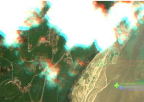
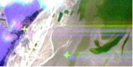
Figure 1: Section2.1×1.5km from a RapidEye scene of southern bavaria (north of F¨ussen) containing clouds and a plane
Fig. 1 shows a part of a RapidEye scene containing clouds and a plane travelling from east to west. The different positions of the
plane in the individual multispectral bands of the sensor is clearly visible. Also the colored border of the clouds is evident. While the different positions of the plane results from a combination of two effects – the movement and the height above ground – the border along the clouds is only due to the height above the ground or more precise: the coregistration plane.
In this paper we show how to exploit this effect in WorldView-2, RapidEye and Pl´eiades imagery to detect and derive moving ob-jects like cars, trains or airplanes from the imagery. In WorldView-2 images cars travelling at a speed of about 60 km/h show a shift of about 4 pixels or 8 meters in the multispectral image between e.g. the green and yellow channel while static objects have shifts below 0.5 pixels (the manually measuring accuracy).
In Rapid-Eye images a plane flying across the acquisition direc-tion of the sensor shows a shift of about 108 pixels or 540 meters between the red and the green band. Between the blue and green band there are still 13 pixels or 65 meters (all measured in or-thorectified imagery). Cars on a highway show up moving about 12 pixels (60 meters) between the green and red band. In the same Rapid-Eye scene clouds show a shift of about 45 meters between the red and green band in acquisition direction. Assum-ing not movAssum-ing clouds allow together with the estimation of the acquisition geometry and -times the estimation of cloud heights. Also – if a plane flies across the acquisition direction – speed and height of the plane are separable and can be retrieved indepen-dently. Planes flying along the acquisition direction mix up these information and for retrieving one the other has to be estimated – e.g. if the height of the plane is estimated the speed may be calculated.
This paper focuses mainly on the estimation of the time gap for the RapidEye sensor since this measure is as unknown as the ex-act focal plane assembly which was extrex-acted from the resulting imagery and some sparse information.
WorldView-2 and Pl´eiades images also a first approach of an automatic de-tection of moving traffic is shown.
1.1 Sensor composition
The WorldView-2 multispectral instrument consists of two CCD lines acquiring in the first the standard channels blue, green, red and the first near infrared band and in the second the extended channels coastal blue, yellow, red edge and the second near in-frared band. These two CCD lines are mounted on each side of the panchromatic CCD line. Therefore the same point on ground is acquired by each line at a different time. Fig. 2 and fig. 3 show the focal plane assemblies (FPA) of WorldView-2 and the Pl´eiades push broom scanner instruments respectively.
Figure 2: Focal plane assemblies of WorldView-2 (sketch cour-tesy Digital Globe)
In table 1 from K¨a¨ab (2011) the time lags for the sensor bands are given.
Table 1: WorldView-2’s recording properties Band recording Sensor Wavelength Inter-band Time lag [s] data order name [nm] Time lag [s] from start Near-IR2 MS2 860-1040 Recording start Recording start Coastal Blue MS2 400-450 0.008 0.008 Yellow MS2 585-625 0.008 0.016 Red-Edge MS2 705-745 0.008 0.024 Panchromatic PAN 450-800
Blue MS1 450-510 0.3 0.324 Green MS1 510-580 0.008 0.332 Red MS1 630-690 0.008 0.340 Near-IR1 MS1 770-895 0.008 0.348
The Pl´eiades FPA is similar but consists only of one multispec-tral and one panchromatic sensor line. The main gap exists only between the multispectral bands and the pan channel where the latter is also mounted in a curvature around the optical distortion center (marked with a×in the figure).
Figure 3: Focal plane assembly Pl´eiades
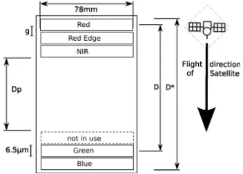
As shown in fig. 4 the RapidEye focal plane assembly consists of five separate CCD lines – one for each band. They are grouped in two mounts: the blue and green on one and the red, red edge and the near infrared band on the second.
Figure 4: RapidEye focal plane assembly (FPA),g: gap between lines,Dp: distance between packages,D∗: maximum distance
between lines,D: distance red–green
So the main gap can be found between the blue/green and the red/RE/NIR bands. The nominal orbit height for RapidEye is given as 630 km. Using the NORAD two-line-elements (TLE) for exact calculation gives an orbit height of 637.5 km. and an average speed of 7.53902 km/s resulting in an orbit of about 97 minutes length.
1.2 Preliminary work
The first one exploiting the time lag between different bands in a very high resolution (VHR) push broom scanner was Etaya et al. (2004). He used QuickBird images of 0.6 m GSD panchro-matic and 2.4 m multispectral and found a time gap between these bands of about 0.2 s.
Also M. Pesaresi (2007) used QuickBird imagery with also a time lag of 0.2 seconds between the panchromatic and the multispec-tral bands.
Tao (Tao and Yu, 2011) proposed 2011 in an IGARSS paper first the usage of WorldView-2 imagery for tracking of moving ob-jects. He calculated from a plane arriving at the Shanghai airport a time delay between the Coastal Blue Band on the second mul-tispectral sensor line and the Blue Band on the first mulmul-tispectral sensor line of about17.5 m/80 m/s = 0.216seconds.
Delvit (Delvit et al., 2012) described in his work on “Attitude Assessment using Pleiades HR Capabilities” the Pl´eiades focal plane (as shown in fig. 3). Here the panchromatic/multispectral shift is significant: 19 mm in the focal plane, which means 1 km on ground or a time delay of 0.15 seconds or in turn also a 1.5 mrad stereoscopic angle. He also describes the maximum offset be-tween two multispectral bands as 6 times smaller (maximum 3 mm). The 1.5 mrad stereoscopic angle means a height of about 300 m corresponds to 0.5 m shift (1 GSD of the pan channel). In turn using a matching accuracy of about 0.1 pixels allow for the ex-traction of a DEM with an uncertainty of 120 m (0.1×4×300m for the multispectral GSD pixel size).
Finally Leitloff (2011) gives in his PHD thesis a short overview of more of these methods and proposed also some approaches for automatic vehicle extraction.
2 METHOD
red and cyan dots. The cars on the highway verify clearly the ac-quisition order: first blue/green and red after the main time gap. This shift is due the car moving some distance (60 m on the high-way) between the acquisition of the bands. A first estimation of the time gap assuming a speed of about 120 km/h on the high-way leads to a relatively large∆tof 1.8 sec which is about ten times the order of the time gaps found in VHR imagery from e.g. QuickBird, WorldView-2 or Pl´eiades.
Figure 5: Principle of acquisition geometry of image bands sepa-rated in a FPA
Since for RapidEye the exact geometry of the focal plane assem-bly (FPA) was not known several approaches were investigated to estimate the time lags between the bands of this satellite:
• Cloud heights – distance between the bands along the flight path measured and the height of the clouds above ground estimated by a highly accurate geometrically simulation of cloud shadows
• Car speeds – distance of cars between bands measured and speed estimated for different road classes
• Plane heights and speeds – distance of planes between bands measured and height together with speed estimated (they are heavily linked together if the plane did not travel exactly across the flight path of the satellite)
Figure 6: Example of moving cars in a RapidEye image (red and cyan dots on the roads)
3 EXPERIMENTS
3.1 Calibration Rapid-Eye – Clouds
The first striking feature looking on a RapidEye image are the red and cyan borders of clouds as can be seen in fig. 8. This is due to the relative large distance of the blue and green to the red CCD array in the focal plane assembly. To exploit this feature for tracking of moving objects this lateral distance of the sensor lines must be converted to a time distance. For all investigations on RapidEye a scene acquired 2011-04-08 11:08:27 over southern Bavaria is used.
A first point of reference is a statement from RapidEye AG itself: “This means that the bands have imaging time differences of up
to three seconds for the same point on the ground,...” (RapidEye (2012), p. 11). Therefore the result for the time delay between the blue and the red band should be approximately 3 seconds.
In general we use for better results of the measurements the dis-tances between red and green band since the green band is less noisy and spectrally closer to the red band.
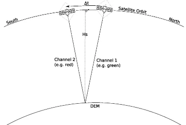
Figure 7: Acquisition geometry of clouds in RapidEye imagery, left: side view, right: top view
In a first step the borders of clouds like in fig. 8 may be used for this purpose. As shown in fig. 7 the (exaggerated) time delay∆t in aquring the same point on a cloud border results in a lateral shift∆son ground in the band-coregistered level-1 images. The time delay∆tmay be expressed as
vs=
∆ss
∆t and ∆ss
∆s =
Hs−hc
hc
⇒∆t=Hs−hc hc
·∆s vs
using the satellite travelling distance∆ssin∆t, the satellite
trav-elling speedvs, the orbit height above groundHsand the cloud
height above groundhc. The satellite height and speed are known
directly from the TLE calculation asHe
s = 631.9km (edenotes
the height relative to the WGS84 ellipsoid, so the satellite height above ground isHs = Hse−h) andvs = 7.53902km/s (see
above). Also the local heighthabove WGS84 ellipsoid is known from a local DEM (see fig. 8, right). So the only remaining un-known value is the height of the cloudhc=hec−h.
Figure 8: Example of a cloud in the RapidEye image near Schon-gau, section3.1×3.1km, left RapidEye image, right ellipsoid DEM ranging from 745 to 845 m (WGS84)
To estimate this height a simulation of a geographic cloud shadow was developed using both the satellite viewing azimuth and inci-dence angles and the sun azimuth and zenith angles.
Fig. 9 shows the cloudmask derived from the image section in fig. 8, left and simulated cloud shadows for different cloud heights he
cranging from 1000 to 2000 m above ellipsoid. As can be seen
in the figure a cloud height on DEM level (h = 800m in this area) will drop no shadow outside of the cloud. Raising the height above the DEM height shifts the cloud shadow to the north east.
Figure 9: Cloud mask from previous image and simulated shadow masks for cloud heights (above ellipsoid) 1000, 1500, and 2000 m
cloud height corresponding to this distance ishe
c= 2019±12m
above ellipsoid orhc = 1219±15m above ground. Using the
satellite height Hs = 631900 m−800 m = 631100 mand
speedvs = 7539m/s together with a measured cloud border of
∆s= 55±10 mgives for the example cloud a
This is nearly 1.3 times the value of 3 seconds as stated by Rapid-Eye. Repeating this procedure for 9 different clouds with clear shadows we gain a statistical result of3.46±0.51seconds for the time lag between the red and the green channel.
3.2 Calibration Rapid-Eye – Cars
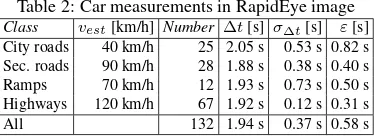
The car measurement follow fig. 6. For the analysis 67 cars on highways, 12 cars on ramps, 28 cars on secondary roads, 25 cars on city roads were measured. The results are:
Table 2: Car measurements in RapidEye image Class vest[km/h] Number ∆t[s] σ∆t[s] ε[s]
The error for the speed estimation was estimated as 20 km/h, the measurement error was estimated as 5 m (1 pixel). Taking into account these estimation and measurement errors together with the statistical errorσ∆tprovides the overall errorεin tab. 2.
3.3 Calibration Rapid-Eye – Planes
Deriving∆tfrom planes is more complicated than using clouds or cars since in flight direction of the satellite also the travelling height of the plane above ground gives an additional shift. As shown in fig. 10 we have to split all distances and also the travel-ling speed of the plane in components across (dc,vc) and along
(da,va) the satellites acquisition directionαs.
The travelling directionˆvof the plane can be derived from the contrails of the planes. Theˆv = (vx, vy)/|(vx, vy)|andd =
(dx, dy) are measured directly from the orthorectified images.
The flight directionαs = 190.56◦of the satellite can be
mea-sured from the orthorectified image on the border or taken from the image metadata (scan azimuth). For the vectors(vc, va)and
analogue for(dc, da)in flight direction helds (the angleαsis a
heading with 0=north, 90=east, . . . therefore the unusual rotation matrix):
Figure 10: Acquisition geometry of planes in RapidEye imagery, left: side view, right: top view
The movement of the plane across the flight directiondcis
inde-pendent of the influence of the FPA and therefore only depending on the speed component in this direction and the time lag∆t between the bands (we take for all measurementsdthe red and green band as stated above):
dc=vc·∆t
In flight direction of the satellite the displacementdais composed
from the speed component in this directionva·∆tand the height
of the plane above ground (see above section “clouds”):
da=va·∆t+ ∆t
Hf−hDEM Hs−Hf
vs
The flight directionsvˆ(heading) and the distancesd= (dx, dy)
were measured directly, the along and across values were calcu-lated usingαs. Tuning the absolute value of the speedvgives
directly the requested∆tand also solving the equation above for Hfthe height above ground of the plane. For the results in tab. 3
we tuned the estimated speeds to give somehow reasonable flight heightsHf of the planes.
Table 3: Plane measurements in RapidEye image,vˆis the head-ing of the plane in degree (north=0, east=90, . . . ),
Nr. vˆ[◦] hDEM[m] d
a[m] dc[m] v[km/h] ∆t[s] Hf[m]
1 348.82◦ 1408 m -865.69 -156.28 500 3.04 11910.54
2 269.40◦ 2195 m -230.54 -591.97 900 2.41 10060.67
3 329.26◦ 1988 m -759.39 -345.49 750 2.51 10430.40
4 17.50◦ 881 m -421.70 -2.40 1000 0.00 ∞ 5 52.50◦ 792 m -727.96 413.35 1050 2.12 9969.70
6 29.91◦ 674 m -458.43 113.11 450 2.73 3533.03
The positions of plane 4 in the red and green band are below 0.5 px in flight direction of the satellite and so below the mea-surement accuracy. For thisdc < εthe∆t = dc/vc = 0and
no heightHfmay be calculated. The resulting times give a mean
∆t = 2.56±0.42s. The measurement error of the position εd= 0.06s, the uncertainty from the speed/height estimation of
εv= 0.23s and the statistical standard deviation ofσ∆t= 0.34s
sum up to an overall error ofε= 0.42s.
3.4 Calibration Rapid-Eye – Relative distances in FPA
Analyzing a flying plane in all five channels of a RapidEye image as shown in fig. 11 let us derive the absolute distances between all channels and also the relative distance of the channels in the FPA (see fig. 4 and tab. 4).
So the assumption for constantg(see fig. 4) between all channels can be assured and a D = dNIR−G + 2g = 8.5gor Dp =
Figure 11: Detailled view of a plane in a RapidEye image, section 1500×750m, all five channels (left to right): red, red-edge (as yellow), NIR (as purple), green, blue
Table 4: Relative distances of bands in RapidEye FPA from plane distance measurements
Bands measured distance[m] relative distanceg R-RE 77.727±3.334 1.032±0.044 RE-NIR 72.482±3.227 0.962±0.043 NIR-G 489.728±3.356 6.503±0.045 G-B 75.718±3.168 1.005±0.042
3.5 Calibration WorldView-2
For WorldView-2 images an absolute calibration of the band time gaps is possible if a stereo image pair acquired within a short time on the same orbit is available. For this analysis we used a WorldView-2 stereo image pair acquired over Munich on 2010-07-12 at 10:29:57 and 10:30:40 respectively or for an interleaved second stereo pair 10:30:16 and 10:30:55. The measurements were done between the first image of 10:29:57 and the third from 10:30:40 or the interleaved second image from 10:30:16 respec-tively.
Figure 12: Time calibration for WorldView-2 stereo imagery; left: a car with positions in red and yellow channel of the first stereo image; right: the same car in the second stereo image
Fig. 12 shows the principle of the absolute calibration using a stereo image pair: For this approach cars are searched in the im-agery for which a constant travelling speed between the acquis-tion of the two stereo images (19 or 43 seconds) is highly prob-able – e.g. on highways. Let the two images be1and3and let the multispectral channels used ber(red) andy(yellow). So we have positions of a carP1r,P1y,P3randP3y. Please remember
the focal plane geometry of WorldView-2: the red and the yellow bands are located in the two different multispectral CCD arrays on each side of the panchromatic CCD array.
For such cars the following travelling speeds can be calculated:
v1=
|P1y−P1r|
∆tyr
, v3=
|P3y−P3r|
∆tyr
,
vy=
|P3y−P1y|
∆t13
andvr=
|P3r−P1r|
∆t13
The time distance between the stereo pair∆t13= 43 sis known while the time distance between the acquisition of the two mul-tispectral CCD arrays∆tyris unknown. Measuring all positions
Pand assuming a constant velocityv=v1=v3 =vy=vrthe
searched∆tyrcan be calculated as
∆tyr=
|P1y−P1r|
v =
|P1y−P1r|
|P3y−P1y|
∆t13
The assumption of constant velocity can be proved coarsly by verifyingv1=v3or|P1y−P1r|=|P3y−P3r|at the both
end-points of the stereo-acquisition. Repeating this measurements for many cars and checking the measured speeds vwith the roads on which the cars are measured for plausibility gives a result of ∆tyr= 0.297±0.085s. The error is resulting from an
inaccu-racy of 1 second in the acquistion times of the images and a mea-surement inaccuracy of 0.5 pixels (or 1 m). This results in an error εvof about 3 km/h in the estimated speed between the stereo
im-ages and such all together a measurement error ofε∆t= 0.062s.
Together with the statistical error ofσ∆t = 0.059s we gain the
overall error ofε= 0.085s. 3.6 Calibration Pl´eiades
The calibration of the Pl´eiades time gap∆tms,panworks in the
same way as for WorldView-2. But here the calculation has to be done between the pan channel and the multispectral chan-nels as shown in fig. 13. For the calibration a multi-stereo image set from Melbourne acquired 2012-02-25, 00:25 was available in the scope of the “Pl´eiades User Group” program. The result for Pl´eiades based on measuring 14 cars is∆tms,pan= 0.16±0.06s
(σ∆t= 0.05s, measurement inaccuracy of 1 m:εd= 0.04s).
Figure 13: Time calibration for Pl´eiades stereo imagery; left: a car with positions in pan and a multispectral channel of the first stereo image; right: the same car in the second stereo image
4 RESULTS
For RapidEye no absolute calibration like for the stereo pairs of WorldView-2 or Pl´eiades is possible. So for the calibration of the RapidEye time gaps many measurements of different car classes (highway, ramps, secondary and city roads), clouds and airplanes are combined for reducing the measurement uncertainties. In a whole 67 cars on highways, 12 cars on ramps, 28 cars on sec-ondary roads, 25 cars on city roads, 9 clouds and 5 valid airplanes are measured. Combining all these results together (see tab. 5) with all estimated, measurement and statistical errors reveil for the big time gap between the red and green channel ∆trg =
2.65±0.50s and for the small gapsga∆tg = 0.41±0.10s.
Table 5: Measured∆trgfor RapidEye using different methods
Method Number ∆trg[s] ε∆t[s]
Clouds 9 3.46 s 0.51 s Cars 132 1.94 s 0.58 s Planes 5 2.56 s 0.42 s All 3 2.65 s 0.50 s
∆trb = ∆trg+ ∆tg = 3.06s matches very well the stated 3 s
in RapidEye (2012).
For WorldView-2 the absolute calibration from the stereo image pair gives∆tyr = 0.297±0.085s and for Pl´eiades∆tms,pan=
0.16±0.06s. Comparing these results to results given in the literature shows a good congruence: Tao and Yu (2011) gave for WorldView-2∆tcb= ∆tyrof 0.216 s (measured from only one
single plane) and K¨a¨ab (2011) a∆tyr = 0.340 s−0.016 s =
0.324s (time lags from start of recoding for yellow and red) where Delvit et al. (2012) stated∆tms,pan= 0.15s for Pl´eiades.
5 CONCLUSION AND OUTLOOK
In this paper we presented a new method for exploiting the special focal plane assembly of most earth observation satellites based on push broom scanners to extract moving objects from only one single multispectral image. For deriving the correct speed of the detected moving objects the exact time gap between the acqui-sitions of the different bands used has to be known. For Rapid-Eye this time was estimated using moving cars, cloud heights and planes. For satellites capable of aquiring short-time in orbit stereo images like WorldView-2 or the new Pl´eiades system an absolute calibration of the inter-band time gap of one image is possible from using a stereo pair.
Implementing this method the whole traffic flow of a complete satellite scene can be extracted to provide a full large-area situ-ation snapshot as extension to long time but only point wise car measurements of local authorities.
Applying automatic image matching and object detection algo-rithms may help in future to speed up the process of large area traffic monitoring from satellites and is subject to future investi-gations.
REFERENCES
Delvit, J.-M., Greslou, D., Amberg, V., Dechoz, C., Delussy, F., Lebegue, L., Latry, C., Artigues, S. and Bernard, L., 2012. Attitude Assessment using Pleiades-HR Capabilities. In: In-ternational Archives of the Photogrammetry, Remote Sensing and Spatial Information Sciences, Vol. 39 B1, pp. 525–530.
Etaya, M., Sakata, T., Shimoda, H. and Matsumae, Y., 2004. An Experiment on Detecting Moving Objects Using a Single Scene of QuickBird Data. Journal of the Remote Sensing So-ciety of Japan 24(4), pp. 357–366.
K¨a¨ab, A., 2011. Vehicle velocity from WorldView-2 satellite imagery. In: IEEE Data Fusion Contest, Vol. 2011.
Leitloff, J., 2011. Detektion von Fahrzeugen in optischen Satel-litenbildern. PhD thesis, Technische Universit¨at M¨unchen.
M. Pesaresi, K. Gutjahr, E. P., 2007. Moving Targets Veloc-ity and Direction Estimation by Using a Single Optical VHR Satellite Imagery. In: International Archives of Photogramme-try, Remote Sensing and Spatial Information Sciences, Vol. 36 3/W49B, pp. 125–129.
RapidEye, 2012. Satellite Imagery Product Specifications. Tech-nical report, RapidEye.
Tao, J. and Yu, W.-x., 2011. A Preliminary study on imaging time difference among bands of WorldView-2 and its potential applications. In: Geoscience and Remote Sensing Symposium (IGARSS), 2011 IEEE International, Vol. 2011, pp. 198–200.
ACKNOWLEDGEMENTS