THE EFFECT OF WEATHER AND TEMPORAL
VARIATIONS ON CALLS FOR POLICE SERVICE
Ellen G. Cohn
Florida International UniversityINTRODUCTION
The belief that weather conditions such as temperature, rainfall, sunlight and humidity affect people’s actions is widespread (see for example, Anderson, 1987; Baron and Bell, 1975, 1976; Dexter, 1904; Feldman and Jarmon, 1979; Harries and Stadler, 1983, 1988; Morrison, 1891; Quetelet, 1842; Rotton and Frey, 1985). In addition, other researchers have found that human behavior is affected by a variety of temporal variables, such as time of day, day of the week, the occurrence of holidays, or even the ever-changing phases of the moon (see for example, Amir, 1971; Falk, 1952; Feldman and Jarmon, 1979; LeBeau and Langworthy, 1986; Lieber and Sherin, 1972; Michael and Zumpe, 1983; 1986; Perry and Simpson, 1987; Tasso and Miller, 1976; Wolfgang, 1958).1
the physical and social environment. Traditional criminological variables such as age, gender, race, unemployment and socioeconomic status cannot adequately explain variations in crime over short-term periods. It appears that the prediction of crime rates over short periods of time may require a different, more widely varying set of predictor variables.
The main focus of this research is to develop a method for predicting such short-term variations in calls for police service (CFS). Because the emphasis is prediction, rather than an attempt to build a theory which will explain why certain behavior patterns are influenced by changes in weather patterns or temporal variations, this research may be unique. Few researchers have attempted to predict short-term variations in crime rates, and those who have tried have not used such a wide range of predictor variables as have been employed here.
THEORETICAL BACKGROUND
Traditionally, theories of crime and criminal behavior have tended to focus on the individual, with an examination of social bonds, individual personality traits, and so on. Recently, however, some criminological researchers have begun to examine the influence of the specific environmental situation and the context of offending on criminal activities (e.g. Clarke and Cornish, 1985), while others are considering routine activities as a possible explanation of criminal behavior (e.g. Cohen and Felson, 1979). This recent work focusses on variations between locations and settings, rather than between individuals, and the basic approach is to examine why criminal eventsoccur, rather than why an individualdevelops into a criminal.
motivations involved and the behaviors required may differ greatly with the type of crime.
Although rational choice theory-based models of offender decision making have not specifically included weather variations or temporal variables, routine activities theory (e.g. Cohen and Felson, 1979) has considered the relationship between some of these variables and criminal behavior. This theory suggests that the organization of society around time-bound activities influence an individual’s opportunities and choices regarding criminal behavior (Felson, 1986). Effectively most people’s behaviors, activities and daily habits fall into regularly repeated patterns which occur so frequently as to become a basic part of everyday life. However, changes in the surrounding environment may alter these patterns; weekly and seasonal cycles, special events and the occurrence of national or local holidays may result in changes in an individual’s pattern of routine activities. Similarly, adverse or especially pleasant weather conditions may result in changes of normal behavior and activities. For example, inclement weather, such as cold temperatures or heavy rainfall, may reduce the number of available victims, as people frequently tend to stay off the street during bad weather.
Changes in the amount of light or darkness present may also influence variations in criminal behavior. In addition to the belief that crime increases at night because darkness may act as a conditioned disinhibitor (Page and Moss, 1976), it has also been pointed out that light/dark variations may have biological effects on individuals. There is some evidence that certain biological processes are photoperiodic (e.g. Rotton and Kelly, 1985). For example, there is a clear diurnal cycle (with a night peak) in the level of plasma testosterone, a male hormone which may be positively related to various aspects of aggressive and antisocial behavior (Olweus, 1987; Schalling, 1987). Seasonal affective disorder (SAD), “a condition characterized by recurrent depressive episodes that occur annually” (Rosenthal et al., 1984:72), provides additional evidence of links between the physical environment (particularly environmental lighting) and human behavior. Wehr and Rosenthal (1989) have pointed out that “changes in the physical environment may precipitate affective episodes” (p.833), which may include manic periods as well as depression, and may contribute to criminal behavior.
possible biological links. Any theory of criminal behavior that aims to be complete and comprehensive would obviously be enhanced by the inclusion of temporal and weather variables. The remainder of this article investigates how far these variables can predict short-term variations in criminal behavior.
THE CURRENT RESEARCH
This research examines the association of weather and temporal variables with the total set of calls for police service (CFS) received by police in Minneapolis, Minnesota. The eventual goal of this line of research is to develop an instrument that will make it possible to predict short-term variations in CFS over time. Such an instrument could be useful both to criminal justice professionals and to the population in general. The main emphasis of this work, therefore, is prediction, rather than an attempt to build a theory that will explain why certain types of behavior are more or less influenced by changes in weather patterns or temporal variations. It is this goal which makes this research unique; few researchers have attempted to predict short-term variations in crime rates, and those who have tried have not used such a wide range of predictor variables as have been employed here.
THE DATA
The weather variables examined in this research included ambient temperature (in degrees Fahrenheit), wind speed (in knots), relative humidity, the presence or absence of precipitation (rain, drizzle, snow, etc.) and the presence or absence of fog or haze. Other variables (such as sky cover and visibility) were originally considered, but had to be eliminated due to problems of multicollinearity.
The temporal variables examined included the time of day (in three-hour blocks), the day of the week,4the month, the presence of light, the occurrence of major holidays, minor holidays and local festivals, and public high school closings. The first day of the month was also examined, as it has been suggested that certain types of crimes (particularly assault, robbery and domestic abuse) increase on the day of arrival of Welfare and AFDC checks (Cohn, 1991). Table 2 includes definitions and sources of all variables, as well as an explanation of the coding process used.
THE ANALYSIS
The method of analysis used was forward multiple linear regression (MLR). The dependent variable was the number of CFS in a
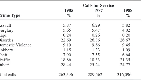
Table 1
CALLS FORSERVICE BYCRIMETYPE
Calls for Service
1985 1987 1988
Crime Type % % %
Assault 5.87 6.29 5.82
Burglary 5.65 5.47 4.02
Rape 0.24 0.26 0.20
Disorder 22.69 26.86 26.67
Domestic Violence 9.19 9.66 9.45
Robbery 1.15 1.33 1.09
Theft 7.90 7.55 6.64
Traffic 18.86 18.33 21.35
Othera 28.44 25.24 24.77
Total calls 263,596 289,562 316,096
given three-hour period. A regression was run on a data set consisting of the 1985 and 1987 CFS data, and the resulting prediction equation was tested on the 1988 data set; this effectively acted as a validation sample to produce an unbiased estimate of the predictive efficiency of the equation (see Cohn, 1991; Farrington and Tarling, 1985). The methodology is in itself a strength of the research, as many of the earlier research used little
Table 2 THEVARIABLES
1. Crime variables– total calls for service Source: MPD call for service data
2. Temporal variables Month of the year Time of day Day of week
aFirst day of the month
Source: MPD call for service data Light
Source: The Astronomical Almanac
Coded: 1 = no light (the entire time period occurred during the night) Coded:2 = mixed (sunrise/sunset occurred during this time period) Coded:3 = daylight (the entire time period occurred during the daytime)
aMajor holidays
(including New Year’s Day, Memorial Day weekend, Independence Day, Labor Day weekend, Thanksgiving Day weekend, Christmas Eve, Christmas Day, New Year’s Eve)
aMinor holidays
(including Valentine’s Day, President’s Day weekend, St Patrick’s Day, Columbus Day, Halloween, Veteran’s Day)
aLocal festivals
(including Winter Carnival, Aquatennial, Minnesota State Fair, 1987 World Series)
aSchool closings (weekdays on which public high schools were closed)
Source: Minneapolis School Board
3. Weather variables
Ambient temperature (degrees Fahrenheit) – squared Wind speed (knots) – squared
Relative humidity – squared
aPrecipitation (rain, snow, sleet, hail, thunderstorms, drizzle, etc.) aFog – fog, dust, smoke, haze, etc.
Source: National Weather Service
or no advanced statistical techniques and frequently ignored problems such as nonlinearity or multicollinearity.
MLR works best with explanatory variables that are not highly intercorrelated (Blalock, 1979). However, collinearity is a frequent problem when using nonexperimental social science data, particularly when polynomial models are used (Neter et al., 1983). The correlations between the explanatory variables in the 1985 data were examined. The majority of the intercorrelations were found to be relatively small (r< 0.4).5In cases of Pearson values greater thanr= 0.4, variables were recoded or combined whenever possible to reduce the correlation. If necessary, variables were dropped from the analysis. For example, sky cover and visibility were highly correlated, both with each other and with precipitation and fog. Recoding did not adequately reduce the intercorrelations, so for both practical and theoretical reasons it was decided to retain rain and fog, and to drop the other variables.6
Basic multiple linear regression assumes a straight line relationship, and does not automatically allow for curvilinear relationships. Criminologists working in this field have rarely given thought to this problem; most (with the notable exception of Rotton and Frey, 1985) have tended to use simple ordinary least squares regression and to ignore the presence of any nonlinear relationships (as, for example, the relationship between CFS and time of day).
Ott (1993) has stated that “re-expressing the...independent variable can transform a nonlinear model into the framework of a linear regression model for some variables”. In this situation, those ratio level explanatory variables which displayed curvilinear relationships with crime (specifically ambient temperature, relative humidity and wind speed) could be transformed, or re-expressed, in such a way as to linearize the data. As the scatterplots all suggest downward curves, the desired transformation on the explanatory variable, according to Ott, would be to use a second or third order polynomial. Neter et al. (1983:305) have pointed out that “fitting of polynomial regression models presents no new problems since...they are special cases of the general linear regression model”. Thus, each of the three ratio-level weather variables was transformed by the use of the squared term.
these coefficients are unsuitable as prediction models. The use of individual dummy variables, such as those that would be used to produce the sheaf coefficients, would result in prediction equations, but the number of dummy variables required would be prohibitive. However, the production of sheaf coefficients7could be used to develop dichotomous variables for time of day, day of week and month. The regression equations produced for each sheaf coefficient show the relative importance of each month, day and time period dummy variable. Examination of the size and direction of the beta weights and correlation coefficients show which are most important to the occurrence of CFS events. The sheaf coefficients were created using the 1985/1987 data, and the beta weights and correlation coefficients from the regression equations determined the exact construction of the three new dichotomous variables. The sheaf coefficients for the day of the week showed that Friday and Saturday were positively correlated with the dependent variable, while the remaining days (including Sunday) were negatively correlated. Therefore, the day of week variable divided the week into “weekend” (Friday/Saturday – coded 1) and “not weekend” (Sunday-Thursday – coded 0). Similarly, the month variable divided the year up into “spring/summer” (May-September – coded 1) and “fall/winter” (October-April – coded 0). Finally, the time of day variable was divided into “morning” (03.00-11.59 hours – coded 1) and “not morning” (12.00-02.59 hours – coded 0).
The independent variables considered in the final analyses included the squared terms for temperature, wind speed and relative humidity, the dichotomous variables for month, day of week and time of day, the presence of light, the first day of the month, major holidays, minor holidays, local festivals, public high school closings, the presence of precipitation and the presence of fog.
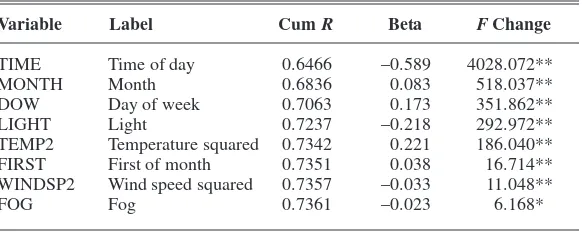
RESULTS
the presence of fog. The cumulative R, the direction of change, the F change and the standardized beta weights for these variables are shown in Table 3.
The resulting prediction equation was validated on the 1988 data set to examine the efficiency of the equation in predicting the total number of calls for service in a future year. The Pearson correlation between the predicted number of calls and the actual number of calls was found to ber= 0.75 (p< 0.01, two-tailed), which was very close to the R value obtained from the 1985/1987 data set.
DISCUSSION
These results suggest that calls for police service are remarkably predictable over short periods of time using temporal and weather variables. The variables most effective in predicting calls for service appear to be temporal variables, especially the time of day, day of the week, month and the presence or absence of light. The direction of the relationships, as indicated by the beta weights, shows that, not surprisingly, calls for service increase during the afternoon and evening hours, on weekends (Friday and Saturday), during the spring and summer months (May through September), and during periods of darkness. These findings are compatible with routine activities theory. LeBeau and Corcoran (1990) have pointed out that “the summer season is warmer, the
Table 3
TOTALCALLS FORSERVICEFINALMODEL– 1985
Variable Label Cum R Beta FChange
TIME Time of day 0.6466 –0.589 4028.072**
MONTH Month 0.6836 0.083 518.037**
DOW Day of week 0.7063 0.173 351.862**
LIGHT Light 0.7237 –0.218 292.972**
TEMP2 Temperature squared 0.7342 0.221 186.040**
FIRST First of month 0.7351 0.038 16.714**
WINDSP2 Wind speed squared 0.7357 –0.033 11.048**
FOG Fog 0.7361 –0.023 6.168*
days are longer, and...more discretionary time is available...” (p. 273). This increase in unstructured time (time not patterned by set recurrent routines and rhythms) may, according to routine activities theorists, result in more opportunities to commit crime. In addition, the warmer temperatures that are present during the summer may also be related to the increase in crime. It might be interesting to learn whether, in countries located in the Southern Hemisphere (where the “summer months” are associated with low temperatures and the “winter months” with warm weather), calls for service still increase during the period between May and September.
The first day of the month is also a significant predictor of calls for police service. An examination of the mean number of calls for service on the first day of the month as compared to all other days shows a distinct increase in the former. The variable for the first of the month is a representation of the arrival of Welfare, AFDC, and other government aid checks. As discussed above, check arrival may act as a catalyst for certain types of crimes. For example, domestic violence and assault may be affected by check arrival, as members of a household argue over the use of the money. Cohn (1993) has shown that the first day of the month is a significant predictor of calls for police service relating to domestic violence. Robberies and thefts may also tend to increase on the first day of the month because criminals could be more likely to believe that there is something to steal. Frequently, checks are stolen from outside mailboxes or the victim is accosted in the street and the check (or the money obtained after the check has been cashed) is taken. Purse snatching tends to increase at this time of the month as well. In addition, the availability of extra money could be related to an increase in disorder calls (drunks, loud parties, loud music, disturbances, etc.).
Major holidays, minor holidays, local festivals and public school closings did not significantly predict calls for police service. It may be that these variables only influence certain types of crimes, and the use of the total calls for service variable might have masked the more specific effect. For example, Cohn (1993) found that public school closings were a significant predictor of domestic violence but not of rape.
1972; Bell and Baron, 1976), which suggested the existence of a curvilinear (inverted-U) relationship between negative affect (produced in some cases by increasingly high ambient temperatures) and aggression. However, Anderson and Anderson (1984) and Anderson (1987) have discussed several serious methodological flaws with this research, mainly relating to the facts that the subjects are aware of their participation in the research and that the temperature manipulations used in the laboratory are extremely obvious to the subjects. Later laboratory studies by Boyanowsky et al. (1981-82) did not find support for the curvilinear relationship between temperature and aggression (although the temperatures examined by Boyanowsky et al. were slightly lower than those used in the Baron studies, which may account for the varied findings). In addition, the majority of field studies relating temperature to criminal behavior have generally produced results supporting a positive linear relationship. For example, Rotton and Frey (1985) found a general linear relationship between temperature and assaults in Dayton, Anderson and Anderson (1984) found the frequency of violent crimes in Chicago and Houston increased monotonically with ambient temperature, and Cotton (1986) found a positive linear relationship between temperature and violent crimes in Indianapolis. None of the field research has provided any support for a curvilinear relationship such as that postulated by Baron and his colleagues.
One possible explanation for the apparent inconsistency in the findings of the field studies and the laboratory studies may be explained by the different ways subjects experience heat in the different research settings. Although temperatures in the laboratory are held constant, this is not true in the field, where temperature varies during the day, and people can escape it, at least partially, by turning on an air conditioner or obtaining a cool drink. Thus, heat in the field may not be experienced as totally as it is in the laboratory. A possible consequence of this is that, in the earlier field studies, the inflection point for the influence of temperature may not have been reached and only the left (increasing) side of the inverted-U curve may have been explored. Unlike earlier field studies, this research has examined temperatures above 100˚F, and may have thus encompassed the elusive inflection point. However, regardless of the cause, it is clear that the findings of this research may provide significant real world support for the “inverted-U” relationship between temperature and criminal behavior.
decrease during windy periods. This is confirmed by an examination of the mean number of calls for service; wind speed exhibited a negative linear relationship with the mean number of total calls for service, so that there were fewer calls to the police during periods of high winds. This supports the results of earlier research by Rotton and Frey (1985), which found a negative relationship between daily wind speed and daily family disturbance complaints. Rotton and Frey have suggested that these relationships may be mediated by the presence of air pollution, as “...these findings are consistent with the well-known fact that high winds disperse pollutants...” (p. 1216). In addition, the frequency of calls is significantly affected by the presence or absence of fog. The negative beta weights suggest that calls are less frequent when it is foggy, and the mean number of calls showed a decrease when fog was present.
Neither relative humidity nor the presence or absence of precipitation are significant predictors of calls for police service. However, as with several of the temporal variables, it may be that research into specific types of criminal behavior could uncover hidden effects.
CONCLUSION
In general, this research is compatible with the basic premisses of routine activities theory, and includes suggestions as to how the theory might be extended to become even more comprehensive. LeBeau and Langworthy (1986) have stated that “the pursuit of routine activities presents the opportunities and circumstances where calls for police services result” (p.139). The results of this research confirm that calls for police service tend to increase during those periods when individuals are less constricted by habitual routine activities. Criminal behavior is more prevalent after dark, at weekends, and during the spring and summer months (when schools are closed and many people take a vacation from their place of work). Calls for police service tend to increase in pleasant weather, becoming more frequent during periods of warm weather and when it is not windy or foggy, when, as Lab and Hirschel (1988) have pointed out, more people tend to be outside or away from home.
although time of day is implied in Hough et al.’s (1980) model concerning vandalism (the model suggests that one situational factor influencing the decision to commit an act of vandalism is the presence or absence of poorly lit streets; as streets are only lit after dark, this appears to imply that the crime is expected to occur at night), time of day is never specifically considered in this model. Including temporal and weather factors in models of crime prevention might assist in explanations of initial involvement, continuance and desistance, as well as in clarifying the sequence of decision making which leads an individual to commit a particular crime. For example, in Cornish and Clarke’s (1986) event model of burglary, which displays the various choices and decisions which lead a burglar to resolve to commit a burglary and to select a particular target house, the effect of various temporal and weather factors which might influence these decisions could be incorporated into the model. Similarly, while many community crime prevention efforts, such as citizen patrols and neighborhood watch programs, already take temporal factors into account (e.g. citizen patrols generally are more frequent at night and on weekends), including weather variables might increase the efficacy of these programs.
Criminal justice professionals also may find this research to be of practical importance. Determining daily predicted numbers of expected calls for service might assist police departments in developing patrol schedules.8Similarly, the prosecutor’s office might find the information of use. For example, in some jurisdictions arrest is now mandatory in cases of misdemeanor domestic violence. Daily variations in the number of domestic violence events are, of course, common. Thus, if there is a large number of domestic violence calls one evening, the prosecutor’s office may find themselves extremely overworked and understaffed the following morning, and offenders are forced to wait for hours before being seen by a prosecutor. The ability to predict “surges” of criminal events and arrests would allow the prosecutor’s office to make advance preparations and perhaps reduce the waiting time of the offenders and their families.
future. Eventually, it may be possible to develop a two-stage prediction process. The first step would only involve the use of temporal variables in developing equations to predict calls for service. These equations could be used to predict the number of calls for service weeks, or even months, in advance. Such advance predictions could be extremely useful to police departments when developing plans for the scheduling and deployment of officers. Other agencies within the criminal justice system, such as the prosecutors’ office, may find this information equally important. The second stage of the process would include weather forecast data shortly before the day or time in question, and would be used to “fine-tune” the prediction.
This research has examined the effect of temporal and weather effects on the total aggregate of calls for service received by the Minneapolis Police Department (MPD). However, not all types of calls are affected in the same way by the same predictor variables. For example, Cohn’s (1993) research into the effects of temporal and weather variables on calls for service relating to domestic violence and rape found significantly different effects of the same predictor variables on the two types of criminal behaviors. Clearly, a focus on individual offense types is extremely important and future research must include consideration of crime-specific effects of these predictor variables.
In conclusion, it is clear that criminologists have tended to neglect the topic of short-term variation in crime rates and have failed to consider many variables that might explain these fluctuations. This work is an attempt to fill the gap in current criminological research. The results of this work show convincingly that accurate prediction of the overall number of calls for service is possible, using variables related to immediate temporal factors and weather conditions. If future research can succeed in incorporating these findings into explanations of changing crime rates, our efficiency in the areas of crime prediction, control and explanation may be improved significantly.
NOTES
Lawrence Sherman, Steve Gottfredson, Ray Surette and several anonymous reviewers for their comments on earlier drafts of this article.
1. See Cohn (1988; 1991) for detailed discussions of prior research in this field.
2. Data for the year 1986 were omitted due to problems with the computerized data tape.
3. One of the key problems in research on temporal variables and criminal behavior is to measure the time of occurrence of the crime. In the past, researchers have used such diverse measures as the time the police were called to the scene, the time on the police report, the time of death (when studying homicides), and even the time an arrested suspect was charged. However, all of these methods have difficulties. Police may not arrive on the scene of a crime until well after it has been committed; especially in the case of low-priority events there may be a delay of hours or even days between the time the victim telephones the police and the actual arrival of an officer on the scene. In addition, police do not make out reports in all cases, resulting in an unofficial “screening” of events: a comparison of 1986 call data in Minneapolis with Uniform Crime Reportsdata on Minneapolis showed that official crime reports were filed for only 28 percent of calls about rapes and 66 percent of calls about robberies (Sherman et al., 1989). The time of death is also problematic. Wolfgang (1958) reported that, for homicides in Philadelphia, the time between assault and death was less than one hour in only 56 percent of the cases, producing a systematic error bias. Finally, the time of charging implies an arrest, which eliminates all cases not cleared by the police, and has the same systematic error problem found in time of death data. In addition, several crimes committed by the same individual at different times could be cleared by one arrest and charging, and thus be assigned the same time.
computer, thus eliminating the “screening” process found in official crime reports, and capturing events that are not recorded in such reports or even in victimization surveys.
Police call data do have several weaknesses, of course. Calls about crimes may be made mistakenly, or as “practical jokes”, similar to setting off a false fire alarm as a prank. In other cases, a single crime may result in multiple calls to the police (i.e. as neighbors on all sides report a domestic quarrel). If the call record is updated by the dispatcher with additional information received from the officers on the scene, it may erroneously be recorded as a separate call, rather than as a supplement to the original file. In addition, there may be a lag of several hours between the time the crime occurs and the time it is first reported to the police. This delay often varies with the type of crime (e.g. a burglary may occur several hours before the householder returns home to discover and report the crime while an assault or robbery may be reported more promptly). However, this lag would also be present and magnified in any other form of crime data.
Thus, despite the weaknesses discussed above, calls for service appear to provide the most extensive and accurate account of what the police are told about crime by the general public. For the purpose of short-term forecasting of crime, the data are relatively accurate with respect to the time of occurrence, and are probably the most precise data available to the criminologist today.
4. The day of the week was assumed to begin at 3 a.m.
5. Given the large sample size, this level of correlation was considered acceptable (see Blalock, 1979 for a discussion of the effect of sample size on MLR with intercorrelated independent variables).
fog will affect the routine activities of an individual than to suggest that the height of the lowest layer of cloud cover or the visibility at six feet above ground level will have such an influence.
7. The procedure for computing a sheaf coefficient is fairly straightforward. It involves creating a series of dummy variables (for example, six dummy variables for the day of the week), running a multiple linear regression model using only these dummy variables and the dependent variable, saving the predicted values as a new variable, and using this new variable, the “sheaf” in the place of the original nominal-level independent variable. A detailed discussion of this statistical technique is presented in Heise (1972).
8. Some departments, such as the Milwaukee Police Department, already take weekend and evening increases in crime into account when scheduling shifts. The Milwaukee Police Department has developed a “power shift” which runs from 8 p.m. to 4 a.m. and overlaps the night (4 p.m.-midnight) and morning (midnight-8 a.m.) shifts during high-crime hours. However, many police departments do not consider even these basic temporal fluctuations; the standard three-shift plan is still common in many departments.
REFERENCES
Amir, M. (1971), Patterns in Forcible Rape, Chicago, IL: University of Chicago Press.
Anderson, C.A. (1987), “Temperature and Aggression: Effects on Quarterly, Yearly, and City Rates of Violent and Nonviolent Crime”, Journal of Personality and Social Psychology, 42:1161-1173.
Anderson, C.A. and Anderson, D.C. (1984), “Ambient Temperature and Violent Crime: Tests of the Linear and Curvilinear Hypotheses”,Journal of Personality and Social Psychology, 46:91-97.
Baron, R.A. and Bell, P.A. (1975), “Aggression and Heat: Mediating Effects of Prior Provocation and Exposure to an Aggressive Model”, Journal of Personality and Social Psychology, 31:825-832.
Baron, R.A. and Bell, P.A. (1976), “Aggression and Heat: The Influence of Ambient Temperature, Negative Affect, and a Cooling Drink on Physical Aggression”, Journal of Personality and Social Psychology, 33:245-255.
Baron, R.A. and Lawton, S.F. (1972), “Environmental Influences on Aggression: The Facilitation of Modeling Effects by High Ambient Temperatures”, Psychonomic Science, 26:80-82.
Bell, P.A. and Baron, R.A. (1976), “Aggression and Heat: The Mediating Role of Negative Affect”, Journal of Applied Social Psychology, 6:18-30.
Blalock, H.M. Jr (1979), Social Statistics, (Rev. 2nd ed.), New York, NY: McGraw Hill Book Company.
Blumstein, A. (1983), “Prisons: Population, Capacity, and Alternatives”, in Wilson, J.Q. (Ed.), Crime and Public Policy, San Francisco, CA: ICS Press, 229-250.
Boyanowsky, E.O., Calvert, J., Young, J. and Brideau, L. (1981-2), “Toward a Thermoregulatory Model of Violence”, Journal of Environmental Systems, 11:81-87.
Clarke, R.V.G. and Cornish, D.B. (1985), “Modeling Offender’s Decisions: A Framework for Research and Policy”, in Tonry, M. and Morris, N. (Eds), Crime and Justice, Vol. 4, Chicago, IL: University of Chicago Press, 147-185.
Cohen, L.E. and Felson, M. (1979), “Social Change and Crime Rate Trends: A Routine Activity Approach”, American Sociological Review, 44:588-608.
Cohn, E.G. (1993), “The Prediction of Police Calls for Service: The Influence of Weather and Temporal Variables on Rape and Domestic Violence”, Journal of Environmental Psychology, 13:71-83.
Cohn, E.G. (1988), “A Review of the Effect of Climatic and Temporal Variations on Crime”, Unpublished M.Phil. thesis, University of Cambridge Institute of Criminology, UK.
Cornish, D.B. and Clarke, R.V. (1986), “Situational Prevention, Displacement of Crime and Rational Choice Theory”, in Heal, K. and Laycock, G. (Eds), Situational Crime Prevention: From Theory into Practice, London: HMSO, 1-16.
Cotton, J.L. (1986), “Ambient Temperature and Violent Crime”, Journal of Applied Social Psychology, 16:786-801.
Dexter, E.G. (1904), Weather Influences: An Empirical Study of the Mental and Physiological Effects of Definite Meteorological Conditions, New York, NY: Macmillan.
Falk, G.J. (1952), “The Influence of the Seasons on the Crime Rate”, Journal of Criminal Law, Criminology, and Police Science, 43:199-213.
Farrington, D.P. and Tarling, R. (1985), “Criminological Prediction: An Introduction”, in Farrington, D.P. and Tarling, R. (Eds), Prediction in Criminology, Albany: State University of New York Press, 2-33.
Feldman, H.S. and Jarmon, R.G. (1979), “Factors Influencing Criminal Behavior in Newark: A Local Study in Forensic Psychiatry”, Journal of Forensic Sciences, 24:234-239.
Field, S. (1990), Trends in Crime and Their Interpretation: A Study of Recorded Crime in Post War England and Wales, London: HMSO.
Felson, M. (1986), “Linking Criminal Choices, Routine Activities, Informal Control, and Criminal Outcomes”, in Cornish, D.B. and Clarke, R.V. (Eds), The Reasoning Criminal: Rational Choice Perspectives on Offending, New York, NY: Springer-Verlag, 119-128.
Harries, K.D. and Stadler, S.J. (1983), “Determinism Revisited: Assault and Heat Stress in Dallas, 1980”, Environment and Behavior, 14:394-417.
Harries, K.D. and Stadler, S.J. (1988), “Heat and Violence: New Findings from Dallas Field Data, 1980 1981”, Journal of Applied Social Psychology, 18:129- 138.
Heise, D.R. (1972), “Employing Nominal Variables, Induced Variables and Block Variables in Path Analysis”, Sociological Methods and Research, 1:91-97.
Hough, J.M., Clarke, R.V.G. and Mayhew, P. (1980), “Introduction”, in Clarke, R.V.G. and Mayhew, P. (Eds), Designing Out Crime, London: HMSO, 1-17.
LeBeau, J.L. and Corcoran, W.T. (1990), “Changes in Calls for Police Service with Changes in Routine Activities and the Arrival and Passage of Weather Fronts”, Journal of Quantitative Criminology, 6:269-291.
LeBeau, J.L. and Langworthy, R.H. (1986), “The Linkages between Routine Activities, Weather, and Calls for Police Services”, Journal of Police Science and Administration, 14:137-145.
Lewin, K. (1936), Principles of Topological Psychology, New York, NY: McGraw-Hill.
Lieber, A.L. and Sherin, C.R. (1972), “Homicides and the Lunar Cycle: Toward a Theory of Lunar Influence on Human Emotional Disturbance”, American Journal of Psychiatry, 129:69-74.
Michael, R.P. and Zumpe, D. (1983), “Sexual Violence in the United States and the Role of Season”, American Journal of Psychiatry, 140:883-886.
Michael, R.P. and Zumpe, D. (1986), “An Annual Rhythm in the Battering of Women”, American Journal of Psychiatry, 143: 637-640.
Morrison, W.D. (1891), Crime and Its Causes, London: Swan Sonnenschein and Co.
Neter, J., Wasserman, W. and Kutner, M.H. (1983), Applied Linear Regression Models, Illinois: Richard D. Irwin, Inc.
Olweus, D. (1987), “Testosterone and Adrenaline: Aggressive Antisocial Behavior in Normal Adolescent Males”, in Mednick, S.A., Moffitt, T.E. and Stack, S.A. (Eds), The Causes of Crime: New Biological Approaches, Cambridge: Cambridge University Press, 263-282.
Ott, R.L. (1993), An Introduction to Statistical Methods and Data Analysis, California: Duxbury Press.
Page, R.A. and Moss, M.K. (1976), “Environmental Influences on Aggression: The Effects of Darkness and Proximity of Victim”, Journal of Applied Social Psychology, 6:126-133.
Perry, J.D. and Simpson, M.E. (1987), “Violent Crimes in a City: Environmental Determinants”, Environment and Behavior, 19:77-90.
Rosenthal, N.E., Sack, D.A., Gillin, J.C., Lewy, A.J., Goodwin, F.K., Davenport, Y., Mueller, P.S., Newsome, D.A. and Wehr, T.A. (1984), “Seasonal Affective Disorder: A Description of the Syndrome and Preliminary Findings with Light Therapy”, Archives of General Psychiatry, 41:72-80.
Rotton, J. and Frey, J. (1985), “Air Pollution, Weather, and Violent Crimes: Concomitant Time Series Analysis of Archival Data”, Journal of Personality and Social Psychology, 49:1207-1220.
Rotton, J. and Kelly, I.W. (1985), “Much Ado about the Full Moon: A Meta-Analysis of Lunar-Lunacy Research”, Psychological Bulletin, 97:286-306.
Schalling, D. (1987), “Personality Correlates of Plasma Testosterone Levels in Young Delinquents: An Example of Person Situation Interaction?”, in Mednick, S.A., Moffitt, T.E. and Stack, S.A. (Eds), The Causes of Crime: New Biological Approaches, Cambridge: Cambridge University Press, 283-291.
Sherman, L.W. (1988), Personal communication.
Sherman, L.W., Gartin, P.R. and Buerger, M.E. (1989), “Hot Spots of Predatory Crime: Routine Activities and the Criminology of Place”, Criminology, 27:27-56.
Tasso, J. and Miller, E. (1976), “The Effects of the Full Moon on Human Behavior”, Journal of Psychology, 93:81-83.
Wehr, T.A. and Rosenthal, N.E. (1989), “Seasonality and Affective Illness”, American Journal of Psychiatry, 146:829-839.