DETECTION OF HARVESTED TREES IN FORESTS FROM REPEATED HIGH DENSITY
AIRBORNE LASER SCANNING
P. J. Pietrzyka,∗, R. C. Lindenberghb a
MSc Geomatics, Delft University of Technology, The Netherlands - [email protected] bDept. of Geoscience and Remote Sensing, Delft University of Technology, 2628 CN Delft, The Netherlands
KEY WORDS:Laser scanning, LIDAR, Change detection, Segmentation, Monitoring, Forestry
ABSTRACT:
Identification of harvested and fallen trees is a prerequisite for the detection and measurement of changes in forests. This paper presents a three step approach to monitor harvested and fallen trees based on direct comparison of repeated high density airborne LIDAR data. In a first step differences between data sets are obtained from a point to point comparison, such that the data can be reduced to the deviating points only. Secondly, the resulting points are clustered into spatially connected regions using region growing. Finally, individual trees are extracted from the clusters by analysing their relative proximity and by analysing geometric properties of points in the clusters. Two data sets, acquired at a four year interval and covering a forest with mainly deciduous trees, are compared. First results show that most points relating to a change can be extracted and that clustering of these with region growing enables us to efficiently separate harvested and fallen trees from the remaining trees. Grouped harvested trees could not be separated using the region growing approach due to touching crowns. Segmentation of these using spectral clustering however identified individual regions well, but the results depend mainly on the pre-defined number of clusters. Crowns of grouped trees can be therefore separated if the number of trees is known.
1. INTRODUCTION
Changes in forest environments are caused by many natural pro-cesses and anthropogenic interventions. Natural propro-cesses range from growth, seasonal variations and competition of individual trees for light and water to disturbances caused by insects, dis-eases and severe weather conditions like heavy wind gusts and snow. Anthropogenic processes include interventions such as clearing, selective removal of individual trees to improve growth of other trees and selective removal of individual branches to avoid branches falling down or to make room for paths. Due to their occurrence at different spatial and temporal scales, from small to large and from gradual to abrupt respectively, the de-tection and measurement of changes in forest cover and canopy structure by means of remote sensing remains a challenging task.
In contrast to data from optical sensors, which provide only two-dimensional information, airborne laser scanning (ALS) data pro-vide both horizontal and vertical information. Because of this three-dimensional nature, ALS data is well suited to detect chan-ges in forest cover and canopy structure. The principle of ALS is based on range measurements from an aircraft or helicopter com-bined with the determination of its position and attitude using a differential Global Positioning System (GPS) and Inertial Mea-surement Unit (IMU) (Wehr and Lohr, 1999). Modern multiple return and full-waveform laser scanners are capable of generating point clouds with high densities of 100 points/m2 and more de-pending on the scanner settings and flight altitude. Such scanners can provide very detailed three-dimensional information on the structure of trees and forests. If the point density is sufficient to obtain a full vertical point distribution at individual tree level, this information can be also used to delineate individual trees (Rah-man and Gorte, 2008, Reitberger et al., 2009, Hu et al., 2014) and to extract detailed information about individual trees such as skeletons and the diameter at breast height (Bucksch et al., 2014). Likewise, by extracting the crown base height, it was shown by Popescu and Zhao (2008) that the vertical point distribution can
∗Corresponding author.
be used to extract tree parameters below the canopy surface. Fur-ther, changes in forests can be detected even at low point densities by matching the histograms of the vertical point distribution from repeated airborne laser scans (Næsset and Gobakken, 2005, Yu et al., 2006). Thus, ALS data provides not only information on the canopy surface but also on the tree structure below it.
However, studies on changes and dynamics in forests derived from ALS data are so far still limited due to the limited amount of multi-temporal ALS datasets. In addition many of these studies use point clouds with relatively low point densities of approx-imately ten (Yu et al., 2004) or less points per square meter (Vastaranta et al., 2012, Vepakomma et al., 2008). Most of such studies use canopy height models (CHM) to derive changes in height, to detect harvested or fallen trees and to study tree gap dynamics. The use of CHMs is practical in most applications as it reduces the amount of data and therefore benefits simplicity and efficiency, but it does not exploit the full content of informa-tion. In addition, the actual tree height is often underestimated in ALS based tree height assessments due to under-sampling, which can be only partly corrected by regression models (Leeuwen and Nieuwenhuis, 2010). Smaller trees, such as suppressed or inter-mediate trees, might not even be represented in a CHM because their crowns are partly or totally covered by crowns of more dom-inant trees. The potential of three-dimensional ALS data to detect changes in forests is thus often not realized. It has been therefore suggested to use the full height distribution of multi-temporal ALS data to detect changes in forests, such as fallen trees, de-foliation and thinning, more reliably (Vastaranta et al., 2012).
In response to advancements in technology, which make high density and multi-view ALS data available, and the ineffective-ness of CHMs to exploit the full information in ALS data we assess in this paper how the whole available vertical distribution can be used to detect harvested and fallen trees. Similar to the efficient analysis of CHMs the use of all data points for change detection must not be downgraded by slow and intensive process-ing. Since the data is of high density, efficient data structures must be used.
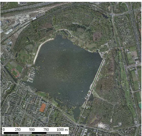
Figure 1: Aerial image of Kralingse Bos (Source: Municipality of Rotterdam)
2. DATA AND TEST SITE
2.1 Test Site
The study area is the Kralingse Bos, a forested area of about one km2in size and located in Rotterdam in the Netherlands, see Fig-ure 1. The area is flat with elevations ranging from three meters below to one meter above mean sea level. The trees are mainly deciduous containing several species including poplar, willow, oak, European beech, maple, European hornbeam and European ash. Tree heights range from approximately 15 to 40 m. The area is a sustainably managed, recreational and urban forest. The management of the forest has changed from a more traditional ap-proach, which included removal of coarse dead wood and dying trees and branches, to the current more sustainable approach. The forest is characterized by multiple layers of canopy and trees of different ages. Decaying fallen trees and branches are left on the ground, giving substrates for insects, bacteria, fungi and mosses, and thereby helping to maintain biodiversity.
2.2 Laser Scanning Data
Two ALS data sets, made available by the municipality of Rotter-dam, are used for this study. The first data, which was acquired in fall 2008 during leaf-on conditions, has a density of about 30 to 50 pulses/m2and due to multiple returns per pulse resulted in up to 200 points/m2. The system scans in front of, below and be-hind the platform to reduce occlusion effects. Furthermore, cross-strips were acquired over the whole area. The second data set was acquired in spring 2012 during leaf-on conditions in cross-strips with a full-waveform scanner and was subsequently discretized; see Figure 2 for a digital surface model derived from the data set. The density is approximately 50 pulses/m2, which, similarly to the first data set, resulted in up to 200 points/m2in the forested area.
3. METHOD
In this section the process to detect harvested and fallen trees is presented. The basic idea of the method is based on a direct com-parison of the raw point clouds with subsequent segmentation and
Figure 2: Digital surface model showing the elevations in the Kralingse Bos in the year 2012
classification. The process is therefore divided into three compo-nents:
1. Deviating points are determined individually using a modi-fied cloud to cloud comparison, which identifies differences between the data sets.
2. The deviating points are further clustered into spatially con-nected regions.
3. The clusters are classified into objects, such as harvested trees, undergrowth or noise.
3.1 Identification of Deviating Points
First, the differences between the two point clouds from the dif-ferent epochs are identified by means of a modified point to point comparison. The essence of our metric is based on the mean of distances from a point in the first epoch to itskclosest points
in the second epoch, which serves as the reference. This dis-tance, which is equivalent to the Hausdorff distance described in Girardeau-Montaut et al. (2005) ifkequals one, can be computed
for each point of the first epoch with respect to the second epoch and is indicative of changes between both epochs. A low value of this distance indicates that no change has occurred, while a large value indicates that there has been a change. For example, points in the first data set, which belong to a tree that exists in the first data set but not in the second, will have a large distance. For these points the closest points in the second data set will in fact belong to structures that still exist, like the ground or neighbouring trees, which, however, might be far away.
To identify changes more robustly our distance is not computed as the distance to the single closest point only, but instead as the mean of distances to thekclosest points, wherekis a user
de-fined parameter larger than one. Even though this distance au-tomatically increases for all points ask is increased, it gives a
To separate changes from non-changes a threshold is defined for the robust cloud to cloud distance, such that points with a value above this threshold are classified as change. All remaining points are not considered to be changes and belong to the same object in the reference epoch. Rather than using a unique threshold for all points in the data set, which would give a noisy result if set too low and exclude changed objects or parts of changed objects if set too high, the threshold includes two components, a unique global and a variable local parameter.
The local parameter is calculated as follows. For each individual data point in the first data set thekclosest points in the second
data set are considered. At each of thesekpoints the mean of the
distances to itsknearest neighbours in its own, i.e. the second,
data set is calculated. We further take the mean of these values; thus overall the mean ofk2distances. The local parameter thus depends on the local spread between points in the reference data, making it adaptable to variations in point density caused by ei-ther the scanning or the object geometry. It can be understood as a normalization distance for our robust cloud to cloud distance. The local threshold further adapts automatically to increases in the robust cloud to cloud distance caused by choosing larger num-ber of closest pointsk. The second component of the threshold,
the global parameterT
g, is a unique user defined value added on
top of the local values and functions solely as a buffer.
The above described method is implemented using a kd-tree data structure to search for nearest neighbours. In this way the neigh-bourhood of each point can be analysed and for each point the robust cloud to cloud distance can be efficiently determined.
3.2 Clustering of Deviating Points
To extract single trees the identified deviating points are first seg-mented into clusters which separate the differences into spatially connected regions. Here region growing is used with the point having maximal robust cloud to cloud distance as seed. Start-ing from this seed the cluster is grown to close-by neighbour-ing points. Close-by neighbourneighbour-ing points are defined as a subset of theknearest neighbours, which must be classified as change
and which are within a distance of one meter to the seed. From these points the cluster is grown further in a similar manner un-til all candidate points are added to the cluster. This procedure is stopped when no more candidate points are available for the cluster. Subsequently a new cluster is grown from the remaining points starting again at the point having the maximal robust cloud to cloud distance as seed. This is iterated until no more points are available as seeds.
3.3 Individual Tree Extraction
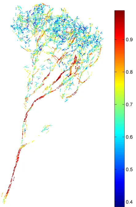
In the last step these clusters are analysed to identify whether they are in fact trees or other objects. All clusters with a low amount of points are removed in order to exclude small objects result-ing either from minor changes, such as small damages to trees, or noise. Further, clusters containing only undergrowth, which can be identified by their low elevation and spatial distribution, are removed. The remaining clusters should be further classified as trees if applicable. It is expected that this can be done using the geometric shape of the clusters and a principal component analysis (PCA) on the neighbourhood of each point to identify stems. A comparable approach has been presented by Bremer et al. (2013) previously. At each point the three eigenvalues and eigenvectors are calculated using a PCA on the coordinates of the point in question and itsknearest neighbours. Due to the
elon-gated and cylindrical shape of stems the points on a stem are char-acterized by a large first eigenvalue compared to the other two
Figure 3: A tree coloured by normalized largest eigenvalue at each point. The arrows depict the directions of the corresponding eigenvectors.
eigenvalues. Further it is assumed that for stem points the largest eigenvalue corresponds to an eigenvector that points in vertical direction. The three eigenvalues of points in tree crowns on the other hand have mainly similar values. As can be seen in Figure 3, a cluster can be classified as a tree if the lower part of that clus-ter consists of points with large first eigenvalue compared to the other two eigenvalues and the corresponding eigenvector point-ing in vertical direction. The upper part of the cluster contains points with a relatively small first eigenvalue that is similar to the other two eigenvalues.
4. RESULTS
The first and second step of the described method have been ap-plied to a subset of the test site covering an area of 100 times 100 m with a high number of removed trees and changes in the undergrowth between the years 2008 and 2012. The correspond-ing results are described in this section. For the classification of individual trees further research is required.
4.1 Identification of Deviating Points
To identify points in the 2008 data, which deviate from the points in the 2012 data, the robust cloud to cloud distance was com-puted, withkset to ten. Similarly the local parameter was
ob-tained by considering the ten nearest neighbours in the 2012 data. The global parameterT
g was set to 0.5 meters. Using this
set-ting the number of points in the 2008 data was reduced from ISPRS Annals of the Photogrammetry, Remote Sensing and Spatial Information Sciences, Volume II-5, 2014
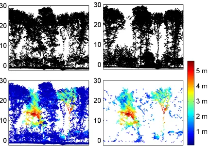
Figure 4: Side view of a small forest patch in 2008 (top left) and 2012 (top right) where two trees have been removed. The robust cloud to cloud distance calculated withk= 10is given in the bottom left and the points identified as change in the bottom right image using
a global thresholdT
gof 0.5 m.
1,146,848, including ground points, to 92,659, thus a reduction of more than 90 percent. These 92,659 points are expected to sam-ple objects that disappeared between 2008 and 2012. The results and the original data for a small forest patch can be seen in Figure 4. In the upper left and right images the cross sections of a small forest patch is presented in the years 2008 and 2012, respectively. A closer look reveals that not only two trees have been removed but also the point density in undergrowth and tree crowns differs. The resulting robust cloud to cloud distance can be seen in the lower left image and shows that for some parts of the removed trees the closest points in the reference data is as far as five me-ters away, which strongly indicates a change. In the lower right image of Figure 4 only the points which remained after applying the threshold are shown. All parts of the removed trees are classi-fied correctly as change, but also some smaller patches from other trees and undergrowth are classified as change. These classifica-tions do not necessarily have to be wrong, but are not desired and therefore have to be removed at a later processing step.
Tests with different values forkshowed that with a low value of koften a relatively small robust cloud to cloud distance is
cal-culated for parts of actually removed trees, where for example undergrowth is close to the stem, where the stem is close to the ground or where the crowns of trees are very dense. A larger value forkreduced this effect slightly. Even though the robust
cloud to cloud distance increases globally for a largerkthe points
corresponding to change can still be isolated from points that do not correspond to changes. To separate the actual change from noise a low value for the global componentT
g of the threshold
was sufficient and can be in the order of half a meter to a meter. If set too low or equal to zero, a large number of points are clas-sified wrongly as change and if set too large real changes might
not be spotted. This is similar to the behaviour of using a unique threshold value for all points, but the two component threshold performs better in areas with changing point densities.
A wide range of effects that can cause differences between the data sets in the tested area are apparent. These range from dif-ferences caused by the natural or anthropogenic changes in the area, like growth, and differences caused by the acquisition like scanning geometry, point density or noise. Nevertheless the most significant large scale changes have been correctly identified us-ing our direct comparison approach.
4.2 Clustering of Deviating Points
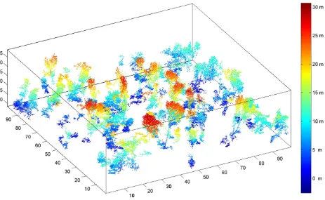
Figure 5: Resulting objects identified as change after region growing and removing of clusters smaller than 100 points. The points are coloured by their elevation.
trees are present including their crown and most of the stem. Sev-eral small patches of undergrowth are still included and should be removed in another processing step.
Next to segmentation by region growing it is proposed to use an approach based on spectral clustering. Here the implementation described by (Chen et al., 2011) will be tested. In this approach the spatial connectedness of neighbouring points is used to seg-ment the point cloud into a predefined number of clusters. First tests have shown that spectral clustering is suitable to delineate neighbouring trees. However the main disadvantages at the mo-ment are the long computation time and the requiremo-ment of know-ing the number of clusters in forehand.
5. CONCLUSIONS
In this paper a method to detect harvested and fallen trees from repeated airborne laser scanning data was presented. In a first step all points that deviate from the reference data were identified, thereby greatly reducing the amount of data for further process-ing. Next, spatially connected points were clustered and small groups of the resulting points are removed. In the final result the removed trees can be identified by a human operator. Further research is however required to learn how the used parameters, like the number of considered closest pointsk, the global
compo-nentTgof the threshold, and the region growing threshold can be
optimized. Further research is also still needed to automatically identify individual trees from the clustering results.
The advantages of the proposed method over methods based on canopy height models are an increase of accuracy due to the ex-ploitation of the three dimensional information in the data and the ability to detect changes below the canopy surface. Consider-ing more than one closest point in the cloud to cloud comparison
and using a local threshold has shown to decrease adverse effects caused by measurement errors, occlusion, varying point densities, effects due to wind or small changes.
In the future the results of the presented method will be validated using small patches in the test site and then applied to the full area. In addition the method will be tested on a data set from 2010, which was acquired during the leaf-off season, in order to test the effect of leaves. It is further planned to compare the obtained results to results from methods based on canopy height models.
ACKNOWLEDGEMENTS
This research is partly funded by the FP7 project IQmulus (FP7-ICT-2011-318787), a high volume fusion and analysis platform for geospatial point clouds, coverages and volumetric data set.
The data for this research has been provided by Stadsbeheer Ge-meente Rotterdam.
REFERENCES
Bremer, M., Wichmann, V. and Rutzinger, M., 2013. Eigenvalue and graph-based object extraction from mobile laser scanning point clouds. ISPRS Annals of Photogrammetry, Remote Sensing and Spatial Information Sciences 1(2), pp. 55–60.
Bucksch, A., Lindenbergh, R., Abd Rahman, M. and Menenti, M., 2014. Breast height diameter estimation from high-density airborne lidar data. Geoscience and Remote Sensing Letters, IEEE 11(6), pp. 1056–1060.
Chen, W.-Y., Song, Y., Bai, H., Lin, C.-J. and Chang, E., 2011. Parallel spectral clustering in distributed systems. Pattern Analysis and Machine Intelligence, IEEE Transactions on 33(3), pp. 568–586.
Girardeau-Montaut, D., Roux, M., Marc, R. and Thibault, G., 2005. Change detection on points cloud data acquired with a ground laser scanner. International Archives of Photogramme-try, Remote Sensing and Spatial Information Sciences 36(part 3), pp. W19.
Hu, B., Li, J., Jing, L. and Judah, A., 2014. Improving the ef-ficiency and accuracy of individual tree crown delineation from high-density lidar data. International Journal of Applied Earth Observation and Geoinformation 26(0), pp. 145 – 155.
Leeuwen, M. and Nieuwenhuis, M., 2010. Retrieval of forest structural parameters using lidar remote sensing. European Jour-nal of Forest Research 129(4), pp. 749–770.
Næsset, E. and Gobakken, T., 2005. Estimating forest growth using canopy metrics derived from airborne laser scanner data. Remote Sensing of Environment 96(3C4), pp. 453 – 465.
Popescu, S. C. and Zhao, K., 2008. A voxel-based lidar method for estimating crown base height for deciduous and pine trees. Remote Sensing of Environment 112(3), pp. 767 – 781.
Rahman, M. and Gorte, B., 2008. Individual tree detection based on densities of high points of high resolution airborne lidar. GEO-BIA pp. 350–355.
Reitberger, J., Schn¨orr, C., Krzystek, P. and Stilla, U., 2009. 3d segmentation of single trees exploiting full waveform lidar data. ISPRS Journal of Photogrammetry and Remote Sensing 64(6), pp. 561 – 574.
Vastaranta, M., Korpela, I., Uotila, A., Hovi, A. and Holopainen, M., 2012. Mapping of snow-damaged trees based on bitemporal airborne lidar data. European Journal of Forest Research 131(4), pp. 1217–1228.
Vepakomma, U., St-Onge, B. and Kneeshaw, D., 2008. Spa-tially explicit characterization of boreal forest gap dynamics us-ing multi-temporal lidar data. Remote Sensus-ing of Environment 112(5), pp. 2326 – 2340. Earth Observations for Terrestrial Bio-diversity and Ecosystems Special Issue.
Wehr, A. and Lohr, U., 1999. Airborne laser scanningłan intro-duction and overview. ISPRS Journal of Photogrammetry and Remote Sensing 54(2C3), pp. 68–82.
Yu, X., Hyypp¨a, J., Kaartinen, H. and Maltamo, M., 2004. Au-tomatic detection of harvested trees and determination of forest growth using airborne laser scanning. Remote Sensing of Envi-ronment 90(4), pp. 451 – 462.