isprsarchives XL 3 W3 399 2015

USE OF VERY HIGH-RESOLUTION AIRBORNE IMAGES TO ANALYSE 3D CANOPY

ARCHITECTURE OF A VINEYARD

S. Burgos a, _{*, M. Mota} a_{, D. Noll} a_{, B. Cannelle} b

a _{University for Viticulture and Oenology Changins, 1260 Nyon, Switzerland} – _{{stephane.burgos, matteo.mota,} dorothea.noll}@changins.ch

b _{School of Engineering and management Vaud (HEIG-VD), 1400 Yverdon, Switzerland - bertrand.cannelle@heig-vd.ch}

KEY WORDS: Vectorization of vine rows, High-resolution DSM, High-resolution images, Drone, UAV.

ABSTRACT:

Differencing between green cover and grape canopy is a challenge for vigour status evaluation in viticulture. This paper presents the acquisition methodology of very high-resolution images (4 cm), using a Sensefly Swinglet CAM unmanned aerial vehicle (UAV) and their processing to construct a 3D digital surface model (DSM) for the creation of precise digital terrain models (DTM). The DTM was obtained using python processing libraries. The DTM was then subtracted to the DSM in order to obtain a differential digital model (DDM) of a vineyard. In the DDM, the vine pixels were then obtained by selecting all pixels with an elevation higher than 50 [cm] above the ground level. The results show that it was possible to separate pixels from the green cover and the vine rows. The DDM showed values between -0.1 and + 1.5 [m]. A manually delineation of polygons based on the RGB image belonging to the green cover and to the vine rows gave a highly significant differences with an average value of 1.23 [m] and 0.08 [m] for the vine and the ground respectively. The vine rows elevation is in good accordance with the topping height of the vines 1.35 [m] measured on the field. This mask could be used to analyse images of the same plot taken at different times. The extraction of only vine pixels will facilitate subsequent analyses, for example, a supervised classification of these pixels.

1. INTRODUCTION

In recent years there has been a growing interest and an increasing number of research studies regarding the application of remote optical and thermal sensing techniques using unmanned aerial vehicle (UAV) in agriculture applications, notably viticulture (Hall et al., 2003, Fiorillo et al., 2012, Mathews & Jensen, 2013). The use of images to map or estimate the growth and water status of plants, or the heterogeneity of different plots have been reported in many papers. Most often different indices like normalized difference vegetation index (NDVI) or other similar combinations of different spectral bands are used. However the analysis of this type of images is difficult in vineyards covered with grass (Santesteban et al., 2013). In that case, the low contrast between the green level in zones under grass coverage and that of vine rows is hardly distinguished with conventional supervised or unsupervised classification. Differencing between green cover and grape canopy is then a challenge for vigour status evaluation. This paper presents the acquisition methodology of very high-resolution (4 cm) images and their processing to construct a 3-dimensional surface model (DSM) for the creation of precise digital surface and terrain models in order to separate the different strata of a vineyard (Zarco-Tejada et al., 2013, Zarco-Tejada et al., 2014).

In the first part, the UAV and the photogrammetric process are presented. In a second part, the extraction of characteristics

(rows, foliage…) of vineyard based on 3D information are

presented. The last part presents some results and advantages and inconvenient of our method.

* Corresponding author

2. PHOTOGRAMMETRIC PROCESS

In this part, each step of photogrammetric process is discussed: acquisition system, flight plan, choice of ground control point (GCP), bundle adjustment and DSM and orthomosaic generation.

2.1 Acquisition system

The UAV that was used in this work to obtain RGB images was a senseFly Swinglet CAM (Figure 1). The choice of this model

was made on the basis of its characteristics: weight (less 500 g included camera), autonomy (30 min), fly speed (36 km/h) and single flight coverage ability (6 km2_{). Images taken with UAV} have a resolution of 3000 x 4000 pixels in RGB. The camera is a compact Canon IXUS 220 HS with a CMOS de 12.1 MP sensor and a 24 mm equivalent focal length.

Figure 3. Homogeneous surface with low number of detectable objects

Figure 4. Traditional orthogonal flight plan and 2 perpendicular directions flight plan on quite a homogenous surface.

Figure 5. Examples of GCP (artificial and natural).

2.2 Flight plan

With Swinglet CAM, the flight plan was prepared at the office and upload on the UAV. Pixel resolution was settled at 4 cm which corresponded to a flight height of about 100 m above ground. This permitted to distinguish the bottom rows and to separate vines without significant blur on picture. Lateral and longitudinal overlap of 75 % and 60 % respectively were applied in order to compute bundle adjustment, then a good DSM with dense matching process. Indeed, extraction of homologous points and matching can be difficult with only grass and soil: texture are repetitive and/or unified (Figure 3). An efficient flight plan to have good matching between images is to fly with orthogonal bands (Figure 4). One flight with 2 perpendicular directions was performed in November 2013 on a vineyard with 1.5 meter between the rows and a slope of about 5 %.

2.3 Ground Control Point

Finding identifiable objects to be used as GCP in vineyard is not evident since it is not possible to add artificial marks (target,

painting…) due to agricultural machinery and vegetation that

grows. We used some artificial and natural points whenever it

was possible. For example, the survey area was composed of 130 images covering 12 hectares with 12 GCP found in more than 6 images. In Figure 5, some examples of GCPs are presented.

2.4 Bundle Adjustment

The software used for bundle adjustment is Pix4Dmapper (http://pix4d.com). This software permit to extract interesting points, computing tie point, calibrate camera and bundle

adjustment. It’s a user-friendly and intuitive software which can

be used by a non-expert in photogrammetry as agronomic scientist. In this study the precision after bundle adjustment on tie points is better than 0.5 pixel and 5 cm on GCP.

2.5 DSM and orthomosaic generation

Figure 6. Textured DSM extracted

2.6 Extraction of characteristics on vineyard

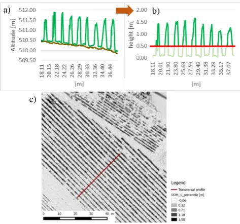
In this study, the position and orientation of vine rows constituted the characteristics to be analysed. To delineate the rows, it was necessary to generate a Digital Terrain Model (DTM) of the ground level of the soil without considering the vegetation height that affects the DSM generated previously. Images were analysed by means of programming with free-use library numpy and GDAL on Python 2.7. The DSM was read as a matrix (numpy.array object) whose elements corresponded to individual pixel elevation using the GDAL library. The second step was performed by applying a 30 x 30 pixel moving window where the minimal, 1 percentile and 5 percentile value of the surrounding pixels replaced the value of the central one. The size of 30 pixel (1.5 m) was chosen to ensure the inclusion of a ground-belonging pixel in the DTM reconstruction, since the rows width was about 40 [cm]. A new matrix was created with the calculated values and replaced into the georeferenced system (Figure 7 a). Then, the DTM was subtracted to original DSM to produce a digital differential model (DDM). The pixels with a difference in altitude higher than 50 cm were extracted using the raster calculator (Qgis 2.8.1) they are assumed to belong to the vine (Figure 7 b and c).

Figure 7: Process of row extraction a) DTM calculation (profile view, braun), b) selection of grape pixels, (profile view), c) visualisation of digital differential model and the transversal

profile (DDM) (aerial view).

3. RESULTS

The Figure 8 shows the 3 DDM obtained with the three different DTMs (minimal, 1 and 5 percentile). The first one (a) used the minimal value and shows quadratic artefacts on pixels with abnormal values. If a pixel shows a very low value, every pixel within the 30 x 30 moving window will inherit the value giving a quadratic artefact. These artefacts disappear when using a 1 (b) or 5 (c) percentile value. The 5-percentile also limits the artefacts but decrease the height of the vine. The influence of such artefacts can be further stated in Figure 9.

Figure 8: Differential model of the vine rows obtained by subtracting the DTM to the DSM. a) Using a minimal filter. b)

Using a 1 percentile filter. c) Using a 5 percentile filter.

Figure 9a shows a transversal cut of two reconstructed DTMs (min and 1 percentile), and Figure 9b shows their corresponding DDMs. Note that the 5-percentile DTM was not included since no additional information was provided. It can be seen that the artefacts lead to an underestimation of the reconstructed ground models, where depression values lead to an over evaluation of the

a) b)

c)

a)

b)

Figure 9 a) Digital Terrain Model reconstructed with minimal value (DTM_min) and 1 percentile value (DTM_per1) b) Digital Differential Model with minimal (min_window) and 1 percentile (1_percentile_window) moving window value.

Figure 10 a) pixels of the DDM with a height > 0.5 [m]. b) RGB image of the same zone. The yellow color correspond to the autumn color of the leaves, before falling.

DDMs, e.g. of the real height of the vine pixels. The pixels located between 9.83 and 11.23 [m] show an aberrant value more than 1 meter lower than the surrounding pixels (Figure 9a) corresponding to an overestimated height vine of 2.5 m (Figure 9b). The use of the 1 percentage value smoothes this noise and does not reduce the height of the rows. The same effect was obtaining by the 5-percentile DTM.

On Figure 10 the comparison of the pixels extracted from the DSM (a) and the RGB image (b) show a very good correspondence. Regarding the validation, an analyse of variance (1 factor ANOVA) on the average height of ten polygons (size bigger than 500 pixels) drawn according to the RGB images on the rows and 10 polygons over the grass cover gave a p value < 0.001 and an average value of 1.23 [m] and 0.08 [m] for the vine and the ground respectively.

4. CONCLUSION

The extraction of the vineyard by using only RGB high-resolution images is often difficult because it depends on combining information from different spectral bands. The colour intensities in each pixel result from merging the images which are not taken with the same incident angle and neither with the same sun elevation. Moreover the colour is not uniform from a grape variety to another, then the thresholds on the RGB layer are difficult to set.

choice of the minimal value of the surrounding pixels. Thus it was possible to extract a digital differential model preventing from the influence of the slope and outliers. In case of a high proportion of outliers the 5-percentile DTM is regarded as more adapted. The manual delineation of vine and grass on the RGB image was used to validate the classification of the pixel according to their height. The average value of 1.23 [m] is in good correspondence with the 1.35 [m] topping height measured on the field.

Within future works the use of the 3D model of the grape canopy will allow a more precise analysis of the vigour status of the plants. The confusion induced by the presence of green cover was largely solved by selecting elevation values instead of colour threshold. The heterogeneity of the plot can then be characterised more efficiently in vineyards with green cover, which tend to become the standard soil surface management system in many wine-growing regions. If the distance between the rows is lower than 1 m or the canopy is not properly developed, in that case production of a DSM becomes difficult on the basis of a 4 cm resolution images. An indirect result is that if there are some holes, foliage is not sufficient and it can be the symptom of a sick vineyard. Therefore the winegrower can go on the field and understand the origin of the problem.

ACKNOWLEDGEMENTS

We thank the University of Applied Sciences of Western Switzerland for funding this research. The project is referenced with number 38333.

REFERENCES

Fiorillo, E., Crisci, A., De Filippis, T., Di Gennaro, S.F., Di Blasi, S., Matese, A., Primicerio, J., Vaccari, F.P., and Genesio L., 2012. Airborne high-resolution images for grape classification: changes in correlation between technological and late maturity in a Sangiovese vineyard in Central Italy. Aust. J. Grape Wine Res., 18(1), pp. 80-90.

Hall, A., Louis J., and Lamb D., 2003. Characterising and mapping vineyard canopy using high-spatial-resolution aerial multispectral images. Comput. Geosci., 29(7), pp. 813-822.

Mathews, A.J., and Jensen J.L.R., 2013. Visualizing and Quantifying Vineyard Canopy LAI Using an Unmanned Aerial Vehicle (UAV) Collected High Density Structure from Motion Point Cloud. Remote Sens., 5(5), pp. 2164-2183.

McGlone, J. C., 2013. Manual of Photogrammetry, Sixth Edition. American Society for Photogrammetry and Remote Sensing (ASPRS), Bethesda, 1372 p.

Santesteban, L.G., Guillaume, S., Royo, J.B., and Tisseyre, B., 2013. Are precision agriculture tools and methods relevant at the whole-vineyard scale? Precis. Agric., 14(1, SI), pp. 2-17.

Zarco-Tejada, P.J., Guillén-Climenta, M.L., Hernández-Clementeb, R., Catalinac, A., Gonzálezc, M.R., Martínc, P., 2013. Estimating leaf carotenoid content in vineyards using high resolution hyperspectral imagery acquired from an unmanned aerial vehicle (UAV). Agric. and Forest Meteorol., 171-172, pp. 281-294.