IMPROVING GOOGLE’S CARTOGRAPHER 3D MAPPING BY CONTINUOUS-TIME
SLAM
Andreas N¨uchtera,b, Michael Bleierb, Johannes Schauera,b, Peter Janottac
a
Informatics VII – Robotics and Telematics, Julius Maximilian University of W¨urzburg, Germany -(johannes.schauer, andreas.nuechter)@uni-wuerzburg.de
b
Zentrum f¨ur Telematik e.V., W¨urzburg, Germany - [email protected] c
Measurement in Motion GmbH, Theilheim, Germany - [email protected]
KEY WORDS:SLAM, trajectory optimization, backpack, personal laser scanner, 3D point clouds
ABSTRACT:
This paper shows how to use the result of Google’s SLAM solution, called Cartographer, to bootstrap our continuous-time SLAM algorithm. The presented approach optimizes the consistency of the global point cloud, and thus improves on Google’s results. We use the algorithms and data from Google as input for our continuous-time SLAM software. We also successfully applied our software to a similar backpack system which delivers consistent 3D point clouds even in absence of an IMU.
1 INTRODUCTION
On October 5, 2016 Google released the source code of its real-time 2D and 3D simultaneous localization and mapping (SLAM) library Cartographer1. The utilized algorithms for solving SLAM in 2D have been described in a recent paper by the authors of the software (Hess et al., 2016). It can deliver impressive results — especially considering that it runs in real-time on commodity hardware. A publication describing the 3D mapping solution is still missing. The released software however, solves the problem. In addition, Google published a very demanding, high-resolution data set to the public for testing their algorithms. Also custom data sets are easy to process, as Google’s software comes with an integration into the robot operating system (ROS) (Quigley et al., 2009). ROS is the de-facto standard in the robotic commu-nity as middleware. It allows to connect heterogeneous software packages via a standardized inter-process communication (IPC) system and is available on recent GNU/Linux distributions.
Google’s sample data set was recorded in the museum “Deutsches Museum” in M¨unchen, Germany. It is the world’s largest mu-seum of science and technology, and has about 28,000 exhibited objects from 50 fields of science and technology. The data set was recorded with a backpack system, which features an iner-tial measurement unit (IMU) and two Velodyne PUCK (VLP-16) sensors. The trajectory we processed was 108 meters long and contained 300,000 3D scans from the PUCK sensors.
Due to a high demand on flexible mobile mapping systems, map-ping solutions on pushcarts, on trolleys, on mobile robots, and backpacks have recently been developed. Human carried systems offer the advantage to overcome doorsteps and that the operator can open closed doors etc. To this end, several vendors build hu-man carried systems which are also often called personal laser scanners.
This paper shows how to use the result of Google’s SLAM solu-tion to bootstrap our continuous-time SLAM algorithm. Our ap-proach optimizes the consistency of the global point cloud, and thus improves on Google’s results. We use the algorithms and data from Google as input for our continuous-time SLAM solu-tion, which was recently published in (Elseberg et al., 2013). We
1https://opensource.googleblog.com/2016/10/ introducing-cartographer.html
present successful applications of the software to our own similar backpack system which delivers consistent 3D point clouds even in absence of an IMU (N¨uchter et al., 2015).
2 STATE OF THE ART 2.1 Laser Scanner on Robots and Backpacks
Mapping environments received a lot of attention in the robotics community, especially after the appearance of cost effective 2D laser range finders. Seminal work with 2D profiles in robotics was performed by Lu and Milios (1994). After deriving 2D vari-ants of the by now well-known ICP algorithm they derived a PosegraphSLAM solution (Lu and Milios, 1997), that considers all 2D scans in a global fashion. Afterwards, many other ap-proaches to SLAM have been presented, including extended Kal-man filters, particle filters, expectation maximization and Graph-SLAM. These SLAM algorithms aimed at enabling mobile robots to map the environments where they have to carry out user spe-cific tasks. Thrun et al. (2000) presented a system, where a hori-zontally mounted scanner performed FastSLAM –a particle filter approach to SLAM– while an upward looking scanner was used to acquire 3D data, exploiting the robot motion to construct en-vironments in 3D. Lu and Milios’ approach was extended to 3D point clouds and poses with six degree of freedom (DoF) in (Bor-rmann et al., 2008).
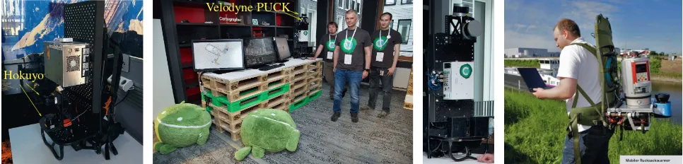
Hokuyo
Velodyne PUCK
Figure 1: Left: Google’s Cartographer system featuring two Hokuyo laser scanners (image: Google blog). Middle: Google’s Cartogra-pher system with two Velodyne PUCKs and the CartograCartogra-pher team (image courtesy of the CartograCartogra-pher team). Right: Second author operating W¨urzburg’s backpack scanner.
and GNSS. In contrast, the Leica Pegasus is a commercially avail-able backpack wearavail-able mobile mapping solution, which is com-posed oftwoVelodyne PUCK scanners, cameras and a GNSS. The PUCKs scan 300.000 points per second and have a maximal range of 100 meters. 16 profilers are combined to yield a vertical field of view of±15 degree.
The Google Cartographer backpack was initially presented in Sep-tember 2014. Back then, the backpack system was based on two Hokuyo profilers and an internal measurement unit (IMU). The current version features two Velodyne PUCK scanners. Figure 1 shows the system from Google and our backpack solution.
2.2 Calibration, Referencing, and SLAM
To acquire high quality range measurement data with mobile laser scanner the position and orientation of every individual sensors have to be known. Traditionally, scanners, GPS and IMU are calibrated against other positioning devices whose pose in rela-tion to the system is already known. The term Boresight cali-bration is used for the technique of finding the rotational param-eters of the range sensor with respect to the already calibrated IMU/GPS unit. In the airborne laser scanning community, au-tomatic calibration approaches are known (Skaloud and Schaer, 2007), and similarly vehicle-based kinematic laser scanning has been considered (Rieger et al., 2010). In the robotics commu-nity there exist approaches for calibrating several range scan-ners semi-automatically, i.e., with manually labeled data (Under-wood et al., 2009) or using automatically computed quality met-rics (Sheehan et al., 2011; Elseberg et al., 2013). Often vendors do not make their calibration methods public and unfortunately, the authors of this paper have no information on the calibration of the Google Cartographer backpack. In general, calibration in-accuracies can to some extend be compensated with a SLAM al-gorithm.
Aside from sensor misalignment, a second source of errors are timing related issues. All subsystems on a mobile platform need to be synchronized to a common time frame. This is often accom-plished with pure hardware via triggering or with mixes of hard and software like pulse per second (PPS) or the network time pro-tocol (NTP). However, good online synchronization is not always available for all sensors. Olson (2010) has developed a solution for the synchronization of clocks that can be applied after the fact. In ROS, sensor data is time-stamped, when it arrives and it is recorded in an open file format (.bagfiles). Afterwards, one works with the time-stamped data using nearest values or inter-polation.
As the term direct referencing or direct Geo-referencing implies, it is the direct measurement of the position and orientation of a mapping sensor, i.e., the laser scanner, such that each range value
can be referenced without the need for collecting additional infor-mation. This means that the trajectory is then used to “unwind” the laser range measurements to produce the 3D point cloud. This approach has been taken by Liang et al. (2014).
Some systems employ a horizontally mounted scanner and per-form 2D SLAM on the acquired profiles. Thrun et al. (2000) used FastSLAM, N¨uchter et al. (2015) used SLAM based on the truncated signed distance function (TSD SLAM), or alternatively, HectorSLAM (Kohlbrecher et al., 2011). These 2D SLAM ap-proaches produce 2D grid maps. Similarly, Google’s Cartogra-pher code is for creating 2D grid maps (Hess et al., 2016). After-wards, the computed trajectory and the IMU measurements are used to “unwind” the laser range measurements to produce the 3D point cloud.
The Google Cartographer library achieves its outstanding per-formance by grouping scans into probability grids that they call submaps and by using a branch and bound approach for loop clo-sure optimization. While new scans are matched with and sub-sequently entered into the current submap in the foreground, in the background, the library matches scans to nearby submaps to create loop closure constraints and to continually optimize the constraint graph of submaps and scan poses. The authors dif-ferentiate between local scan matching which inserts new scans into the current submap and which will accumulate errors over time and global SLAM which includes loop closing and which removes the errors that have accumulated in each submap that are part of a loop. Both, local and global matching are run at the same time.
During local scan matching, the Cartographer library matches each new scan against the current submap using a Ceres-based scan matcher (Agarwal et al., n.d.). A submap is a regular proba-bility grid where each discrete grid point represents the probabil-ity that the given grid point is obstructed or free. These two sets are disjoint. A grid point is obstructed if it contains an observed point. Free points are computed by tracing the laser beam from the estimated scanner location to the measured point through the grid. The optimization function of the scan matcher makes use of the probability grid as part of its minimization function.
traversed using a greedy depth first search and the upper bound of the inner nodes being defined in terms of computational effort and quality of the bound. To compute the upper bound efficiently, grids are precomputed for each height of the tree that overlay the involved submaps and store for each obstructed grid point the maximum values of possible scores. This operation is done in O(n)withnbeing the number of obstructed grid points in each precomputed grid.
Hess et al. (2016) describe the 2D version of the algorithm, which uses the horizontally mounted 2D profiler. The provided data sets contain also data from a setup with Velodyne PUCK scanners (cf. Figure 1 middle). Their algorithm is able to process 3D data and to output poses with 6 DoF, however, a description of their 3D ap-proach is missing from their paper. Nevertheless, we understand from their published source code that their 3D implementation is mostly an extension of their 2D approach to three dimensions with a 3D probability grid. Some changes have been made to improve performance. For example, the 3D grid is not fully tra-versed to find free grid cells but only a configurable distance up to the measured point is checked.
Only a few approaches optimize the whole trajectory in a con-tinuous fashion. Stoyanov and Lilienthal (2009) presented a non rigid optimization for a mobile laser scanning system. They opti-mize point cloud quality by matching the beginning and the end of a single scanner rotation using ICP. The estimate of the 3D pose difference between the two points in time is then used to optimize the robot trajectory in between. In a similar approach Bosse and Zlot (2009) use a modified ICP with a custom corre-spondence search to optimize the pose of six discrete points in time of the trajectory of a robot during a single scanner rotation. The trajectory in between is modified by distributing the errors with a cubic spline. The software of Riegl RiPRECISION MLS automatically performs adjustments of GNSS/INS trajectories to merge overlapping mobile scan data based on planar surface el-ements. Our own continuous-time SLAM solution improves the entire trajectory of the data set simultaneously based on the raw point cloud. The algorithm is adopted from Elseberg et al. (2013), where it was used in a different mobile mapping context, i.e., on platforms like the LYNX mobile mapper or the Riegl VMX-250. As no motion model is required, it can be applied to any continu-ous trajectory.
3 CONTINUOUS-TIME SLAM 3.1 6D SLAM
To understand the basic idea of our continuous-time SLAM, we summarize its foundation, 6D SLAM, which was designed for a high-precision registration of terrestrial 3D scans, i.e., globally consistent scan matching (Borrmann et al., 2008). It is available in3DTK – The 3D Toolkit2. The globally consistent scan match-ing is a full SLAM solution for 3D point clouds.
6D SLAM works similarly to the well-known iterative closest points (ICP) algorithm, which minimizes the following error func-tion
Dare given by minimal distance, i.e.,miis the closest point to
2http://threedtk.de
diwithin a close limit (Besl and McKay, 1992). Instead of the two-scan-Eq. (1), we look at then-scan case
E=X
j→k
X
i
|Rjmi+tj−(Rkdi+tk)|2, (2)
wherejandkrefer to scans of the SLAM graph, i.e., to the graph modeling the pose constraints in SLAM or bundle adjustment. If they overlap, i.e., closest points are available, then the point pairs for the link are included in the minimization. We solve for all poses at the same time and iterate like in the original ICP. The derivation of a GraphSLAM method using a Mahalanobis distance that describes the global error of all the poses
W=X
j,k is the linearized error metric and the Gaussian
dis-tribution is ( ¯Ej,k,Cj,k)with computed covariances from scan matching as given in (Borrmann et al., 2008).X′
jandX ′ kdenote
the two poses linked in the graph and related by the linear error metric. Minimizing Eq. (2) instead of (3) does not lead to differ-ent results (N¨uchter et al., 2010). In matrix notationWin Eq. (3) becomes
W = ( ¯E−HX)TC−1
( ¯E−HX).
HereHis the signed incidence matrix of the pose graph, E¯ is the concatenated vector consisting of allE¯′
j,kandCis a
block-diagonal matrix comprised ofC−1
j,kas submatrices. Minimizing
this function yields new optimal pose estimates.
Please note, while there are four closed-form solutions for the original ICP Eq. (1), linearization of the rotation in Eq. (2) or (3) seams to be always required.
Globally consistent scan matching is a full SLAM solution for 3D point clouds. It is an offline algorithm and thus optimizes
allposes in the SLAM pose graph. As a result, processing more scans will increase the algorithm’s run-time.
3.2 Continuous-time SLAM
We also developed an algorithm that improves the entire trajec-tory of the backpack simultaneously. The algorithm is adopted from Elseberg et al. (2013), where it was used in a different mo-bile mapping context, i.e., on wheeled platforms. Unlike other state of the art algorithms, like (Stoyanov and Lilienthal, 2009) and (Bosse and Zlot, 2009), it is not restricted to purely local improvements. We make no rigidity assumptions, except for the computation of the point correspondences. We require no ex-plicit motion model of a vehicle for instance, thus it works well on backpack systems. The continuous-time SLAM for trajectory optimization works in full 6 DoF, which implies that even planar trajectories are turned into poses with 6 DoF. The algorithm re-quires no high-level feature computation, i.e., we require only the points themselves.
in this fashion. Applying rigid pose estimation to this non-rigid problem directly is also problematic since rigid transformations can only approximate the underlying ground truth. When a finer discretization is used, single 2D scan slices or single points result that do not constrain a 6 DoF pose sufficiently for rigid algo-rithms.
More mathematical details of our algorithm are given in (Else-berg et al., 2013). Essentially, we first split the trajectory into sec-tions, and match these sections using the automatic high-precision registration of terrestrial 3D scans, i.e., globally consistent scan matching that is the 6D SLAM core. Here the graph is estimated using a heuristic that measures the overlap of sections using the number of closest point pairs. After applying globally consistent scan matching on the sections the actual continuous-time or semi-rigid matching as described in (Borrmann et al., 2008; Elseberg et al., 2013) is applied, using the results of the rigid optimiza-tion as starting values to compute the numerical minimum of the underlying least square problem. To speed up the calculations, we make use of the sparse Cholesky decomposition by (Davis, 2006).
Given a trajectory estimate, we “unwind” the point cloud into the global coordinate system and use nearest neighbor search to establish correspondences at the level of single scans (those can be single 2D scan profiles). Then, after computing the estimates of pose differences and their respective covariances, we optimize the trajectory. In a predependend step, we consider trajectory elements everyksteps and fuse the trajectory elements around these stepsltemporarily into a meta-scan.
A key issue in continuous-time SLAM is the search for closest point pairs. We use an octree and a multi-core implementation using OpenMP to solve this task efficiently. A time-threshold for the point pairs is used, i.e., we match only to points if they were recorded at leasttdtime steps away. This time corresponds to the
number of separate 3D point clouds acquired by the PUCKs. It is set to 0.1 sec. (k= 300,l= 300). In addition, we use a maximal allowed point-to-point-distance which has been set to 50 cm.
Finally, all scan slices are joined in a single point cloud to enable efficient viewing of the scene. The first frame, i.e., the first 3D scan slice from the PUCKs scanner defines the arbitrary reference coordinate system.
4 BOOTSTRAPPING CONTINUOUS-TIME SLAM WITH GOOGLE’S SLAM SOLUTION For improving the Cartographer 3D mapping, the graph is es-timated using a heuristics that measures the overlap of sections using the number of closest point pairs. After applying globally consistent scan matching on the sections for several iterations the actual continuous-time SLAM is started.
The data set provided by Google is challenging in several ways: Due to the enormous amount of data, clever data structures are needed to store and access the point cloud. We split the trajectory every 300 PUCK-scans and join±150 PUCK-scans into a meta-scan. These meta-scans are processed with our octree where we use a voxel size of 10 cm to reduce the point cloud by select-ing one point per voxel. We prefer a data structure that stores the raw point cloud over a highly approximative voxel represen-tation. While the latter one is perfectly justifiable for some use cases, it is incompatible with tasks that require exact point mea-surements like scan matching. Our implementation of an octree prioritizes memory efficiency. We use pointers in contrast to se-rialized pointer-free encodings in order to efficiently access the
large amounts of data. The octree is free of redundancies and is nevertheless capable of fast access operations. Our implementa-tion allows for access operaimplementa-tions inO(logn). We use 6-bytes for pointers as this is sufficient to address a total of 256 terabyte. Two bit fields signal if there is a child or leaf node, thus our implemen-tation needs a few bit operations and the 8 byte are sufficient for an octree node.
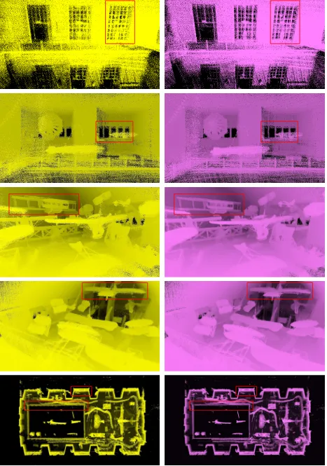
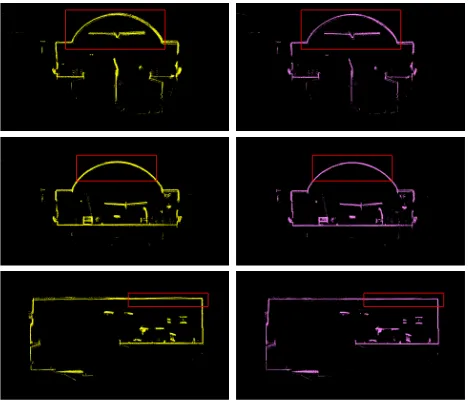
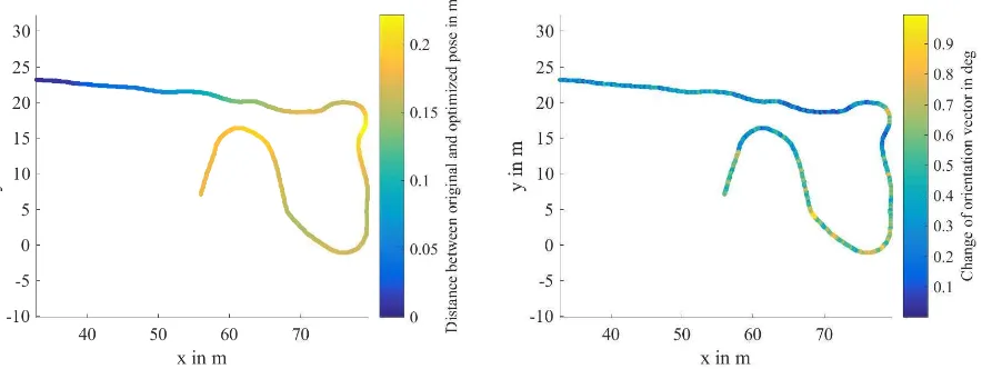
The preprocessing step of the continuous-time SLAM runs for 20 iterations, where the edges in the graph are added, when more than 400 point pairs between these meta-scans are present. The maximal allowed point-to-point distance is set to 50 cm. Figure 3 and present 4 results where the consistency of the point cloud has been improved. Figure 5 shows the modifications in the 3D point cloud, while Figure 6 details the changes in the trajectory’s position and orientation. It is an open traverse, thus the changes are mainly at the end of the trajectory. Processing was done on a server featuring four Intel Xeon CPUs E7-4870 with 2.4 GHz (40 cores, 80 threads). We have optimized the Google data set for 12 to 15 days (few interruptions).
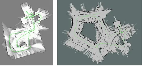
5 FURTHER CARTOGRAPHER SLAM RESULTS In further experiments, we evaluated the Cartographer. As the li-brary is fully integrated into ROS, we are able to exchange on our backpack HectorSLAM or TSD SLAM with Cartographer. In-door office-like environments are no challenge for all the named algorithms. Featureless environments such as long tunnels or out-door environments are problematic. Figure 2 shows a typical er-roneous map obtained with default parameters of Cartographer vs. HectorSLAM in the environment where the photo Figure 1 (right) has been taken.
6 SUMMARY, CONCLUSION AND FUTURE WORK This paper revisits a continuous-time SLAM algorithm and its ap-plication on Google’s Cartographer sample data. The algorithm starts with splitting the trajectory into sections, and matches these sections using the automatic high-precise registration of terres-trial 3D scans.
Needless to say, a lot of work remains to be done. First of all, we plan to evaluate 2D mapping method as we have indicated above. Secondly, as calibration is as crucial as SLAM, we will apply our calibration framework (Elseberg et al., 2013) to the data files pro-vided by Google. Furthermore, we will transfer our continuous-time SLAM to different application areas, e.g., underwater and aerospace mapping applications.
Figure 4: Results of continuous-time SLAM on Google’s Cartographer sample data set Deutsches Museum in M¨unchen. Left: input. Right: output of our solution. Shown are sectional views of the museum hall. Major changes in the point cloud are highlighted in red.
0 0.02 0.04 0.06 0.08 0.1
P
o
in
t-to
-p
o
in
t
d
is
ta
n
ce
in
m
Figure 6: Visualization of the changes in the trajectory computed by our method to bootstraped trajectory. Left: distance. Right: orientation
References
Agarwal, S., Mierle, K. and Others, n.d. Ceres solver. http: //ceres-solver.org.
Besl, P. and McKay, N., 1992. A Method for Registration of 3–D Shapes. IEEE Transactions on Pattern Analysis and Machine Intelligence (PAMI)14(2), pp. 239–256.
Borrmann, D., Elseberg, J., Lingemann, K., N¨uchter, A. and Hertzberg, J., 2008. Globally consistent 3d mapping with scan matching. Journal Robotics and Autonomous Systems (JRAS)
56(2), pp. 130–142.
Bosse, M. and Zlot, R., 2009. Continuous 3D Scan-Matching with a Spinning 2D Laser. In: Proceedings of the IEEE Inter-national Conference on Robotics and Automation (ICRA ’09), pp. 4312–4319.
Chen, G., Kua, J., Shum, S., Naikal, N., Carlberg, M., and Za-khor, A., 2010. Indoor Localization Algorithms for a Human-Operated Backpack System. In: Proceedings of the Interna-tional Conference on 3D Data Processing, Visualization, and Transmission (3DPVT ’10), Paris, France.
Davis, T. A., 2006. Direct Methods for Sparse Linear Systems. SIAM.
Elseberg, J., Borrmann, D. and N¨uchter, A., 2013. Algorith-mic solutions for computing accurate maximum likelihood 3D point clouds from mobile laser scanning platforms. Remote Sensing5(11), pp. 5871–5906.
Hess, W., Kohler, D., Rapp, H. and Andor, D., 2016. Real-time loop closure in 2d lidar slam. In: Proceedings of the IEEE International Conference on Robotics and Automation (ICRA ’16), Stockholm, Sweden.
Kohlbrecher, S., Meyer, J., von Stryk, O. and Klingauf, U., 2011. A flexible and scalable slam system with full 3d motion esti-mation.In: Proceedings of the IEEE International Symposium on Safety, Security and Rescue Robotics (SSRR ’ 11).
Liang, X., Kukko, A., Kaartinen, H., andY. Xiaowei, J. H., Jaakkola, A. and Wang, Y., 2014. Possibilities of a personal laser scanning system for forest mapping and ecosystem ser-vices.Sensors14(1), pp. 1228–1248.
Lu, F. and Milios, E., 1994. Robot Pose Estimation in Unknown Environments by Matching 2D Range Scans.In: Proceedings of the IEEE Computer Society Conference on Computer Vision and Pattern Recognition (CVPR ’94), pp. 935–938.
Lu, F. and Milios, E., 1997. Globally Consistent Range Scan Alignment for Environment Mapping. Autonomous Robots
4(4), pp. 333–349.
N¨uchter, A., Borrmann, D., Koch, P., K¨uhn, M. and May, S., 2015. A man-portable, imu-free mobile mapping system. In: Proceedings of the ISPRS Geospatial Week 2015, Laserscan-ning 2015, ISPRS Ann. Photogramm. Remote Sens. Spatial Inf. Sci., II-3/W5, La Grande Motte, France, pp. 17–23.
N¨uchter, A., Elseberg, J., Schneider, P. and Paulus, D., 2010. Study of Parameterizations for the Rigid Body Transforma-tions of The Scan Registration Problem. Journal Computer Vision and Image Understanding (CVIU)114(8), pp. 963–980.
Olson, E., 2010. A Passive Solution to the Sensor Synchro-nization Problem. In: Proceedings of the IEEE/RSJ Inter-national Conference on Intelligent Robots and Systems (IROS ’10), pp. 1059–1064.
Quigley, M., Gerkey, B., Conley, K., Faust, J., Foote, T., Leibs, J., Berger, E., Wheeler, R. and Ng, A., 2009. Ros: an open-source robot operating system. In: Proceedings of the IEEE International Conference on Robotics and Automation (ICRA ’09), Kobe, Japan.
Rieger, P., Studnicka, N. and Pfennigbauer, M., 2010. Boresight Alignment Method for Mobile Laser Scanning Systems. Jour-nal of Applied Geodesy (JAG)4(1), pp. 13–21.
Saarinen, J., Mazl, R., Kulich, M., Suomela, J., Preucil, L. and Halme, A., 2004. Methods For Personal Localisation And Mapping. In: Proceedings of the 5th IFAC symposium on In-telligent Autonomous Vehicles (IAV ’04).
Sheehan, M., Harrison, A. and Newman, P., 2011. Self-calibration for a 3D Laser. International Journal of Robotics Research (IJRR)31(5), pp. 675–687.
Skaloud, J. and Schaer, P., 2007. Towards Automated LiDAR Boresight Self-calibration.In: Proceedings of the 5th Interna-tional Symposium on Mobile Mapping Technology (MMT ’07).
Stoyanov, T. and Lilienthal, A. J., 2009. Maximum Likelihood Point Cloud Acquisition from a Mobile Platform. In: Pro-ceedings of the IEEE International Conference on Advanced Robotics (ICAR ’09), pp. 1– 6.
Thrun, S., Fox, D. and Burgard, W., 2000. A Real-time Algo-rithm for Mobile Robot Mapping with Application to Multi Robot and 3D Mapping. In: Proceedings of the IEEE Inter-national Conference on Robotics and Automation (ICRA ’00), San Francisco, CA, USA.