Nicoleta Breaz-2. 119KB Jun 04 2011 12:09:17 AM

THE CROSS-VALIDATION METHOD IN THE

SMOOTHING SPLINE REGRESSION

by Nicoleta Breaz

Abstract. One of the goals, in the context of nonparametric regression by smoothing spline functions, is to choose the optimal value for the smoothing parameter. In this paper, we deal with the cross validation method(CV), as a performance criteria for smoothing parameter selection. First, we implement a CV-based algorithm, in Matlab 6.5 medium and we apply it on a test function, in order to emphase the quality of the fitting by the CV-smoothing spline function. Then, we fit some real data with this kind of function.

1.Introduction

We consider the observational regression model,

( )

x i n

f

yi = i +

ε

i, =1, ,

with

ε

=

(

ε

₁,

ε

₂,...,

ε

_n

)

′ ~ N

(

0,

σ

2I

)

and the data,

y

_i, having the weights

0

,

_i

>

i

w

w

. If the plot of data presents some classical trend, as polynomial for example, we choose the parametric regression technique, else, we choose the nonparametric regression technique.

A parametric model is based on some assumed form of the regression function which depends on a finite number of many unknown parameters(see for example, the polynomial regression). In this case, the goal is to estimate these parameters.

By contrast, a nonparametric model doesn’t make assumptions about the shape of the estimator but about the “quality” of the estimator. This quality refers to some general properties as smoothness, for example.

Moreover, if the data are noisy, it is more appropriate to find an estimator that is not very close to data but is sufficiently smooth (see[6]).

Such estimator will minimize, for example, the following expression:

( )

(

)

(

( )

( )

)

[

] [ ]

∑

₌n − +

∫

≥ ⊆

i

b

a m i

i

i y f x f x x x a b

w

1

max min 2

2

, ,

, 0 ,

λ

λ

. (1)

smoothness. If

λ

=0, we obtain the interpolant to the data and if

λ

→∞, we obtain the straight line least squares approximation. Obviously a large value of

λ

leads to a smooth curve but not so close to data and a small value of

λ

leads to a rough curve that follows the data closely .

The expression (1) is often known, as penalized least squares criteria. If we search the solution of this variational problem in some appropriate space, we obtain the estimator called smoothing spline. The name “spline” comes from fact that the estimator is practically, a natural polynomial spline function, of 2m−1 degree (see [3]).

A case of interest is the particular case, m=2, when we obtain as an estimator, the natural cubic spline function. These functions are piecewise-cubic polynomial function, with continuous first and second derivatives, at the break points.

Although the smoothing spline appears in the context of the nonparametric regression, however, the estimator depends on a parameter

λ

, namely, the smoothing spline parameter. There are known several methods to select the smoothing parameters and among these, is cross validation method (CV).

2.The CV-smoothing parameter selection method

When we try to choose the optimal model to data we can use some performance criteria as a testing tool (see [1]). One of these performance criteria is based on a natural way to select that fitting and implicitly, that

λ

, which minimizes the expected prediction error,

( )

(

( )

)

2

x f y E

PSE

λ

= ′− _λ ′ ,

where

x

′

,

y

′

are new data.

Since additional data are not usually available, an estimator of PSE

( )

λ

will be used instead of PSE

( )

λ

. According to [1], one of such estimator is the (leaving-out-one) cross-validation function, given by

( )

∑

(

( )

( )

)

=

−

−

=

n

i

i i i

i

y

f

x

w

n

CV

1

2

1

λ

λ

,

where

f

_λ( )−i is the smoothing spline estimator, fitted from all data, less the i-th data. The (leaving-out-one) cross validation method uses n learning samples, everyone with

1 −

order to validate the models. Since CV

( )

λ

is an estimator for PSE

( )

λ

, a value of

λ

, that minimizes CV

( )

λ

, represents an optimal choice for

λ

.

3.Numerical experiments

In order to show how the CV method works, we implement in Matlab 6.5 medium, the following algorithm, based on CV:

CV-Algorithm

Step 1. Read the sample data

(

xi,yi

)

,i=1,n and if is necessary, order and reweight

the data, in respect with data sites,

x

i. In stead of n1 data,

(

xn₁,yn_1i

)

, with weights

i

n

w

1 ,

i

=

1

,

n

1, we will have just one data,

(

x

n1

,

y

n1

)

, with

∑

∑

= =

= ₁

1 1

1 1

1

1 1

n

i n n

i

n n n

i i i

w y w y

and the weight,

∑

₌

= 1 1 1

1

n

i n n w _i

w .

After this step, the data sites,

x

_i, must be strictly increasing and having the tail n′≤n.

Step 2. For each i,

i

=

1

,

n

′

, determine the cubic smoothing spline,

f

_λ( )−i , based on leaving-out-one resampling method.

Step 3. Calculate the value of the function, CV

( )

λ

. STOP.

Step 4. Calculate CV

( )

λ

, for different values of

λ

.

The appropriate value of

λ

is

λ

CV , with

( )

λ

_λ

CV

( )

λ

CV

CV

=

min

.

If we set

1

0

,

1

<

<

−

=

q

q

q

λ

,

we can search

λ

, by searching q, over a grid on

[ ]

0,1 . In this paper, we use a regular grid, with 1000 points.

Obviously, a large value for q leads to a small value for

λ

and consequently to a rough curve, closely to data points. By contrast, small values for q give large values for

λ

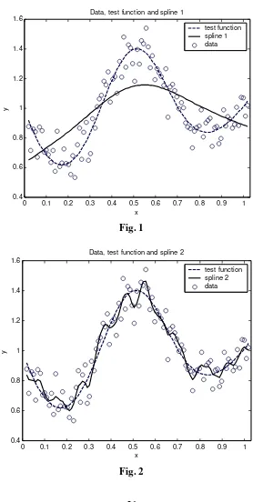
and smooth, but not closely to data, curves.

In that following, we will consider the test function,

( )

2

2 1 20 5

2

3



    − − −

+

+

−

=

x x x x

e

e

x

f

and the noisy data

(

x

_i

,

y

_i

)

,

with

n

i

x

_i

=

,

y

_i

=

f

( )

x

_i

+

ε

_i,

ε

_i

∈

N

(

0

;

0

,

1

)

,

i

=

1

,

100

.

Here

ε

_i,

i

=

1

,

100

, come from a random number generator simulating independently and identically distributed, random variables.

By running the algorithm presented above, for 100 replicates, we obtain an average value

q

_CV

=

0

,

9996

, that leads to

λ

_CV

=

4

⋅

10

−4.

0 0.1 0.2 0.3 0.4 0.5 0.6 0.7 0.8 0.9 1 0.4

0.6 0.8 1 1.2 1.4

1.6 Data, test function and spline 1

x

y

[image:5.595.160.438.82.634.2]

test function spline 1 data

Fig. 1

0 0.1 0.2 0.3 0.4 0.5 0.6 0.7 0.8 0.9 1

0.4 0.6 0.8 1 1.2 1.4 1.6

x

y

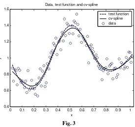
Data, test function and spline 2

test function spline 2 data

0 0.1 0.2 0.3 0.4 0.5 0.6 0.7 0.8 0.9 1 0.4

0.6 0.8 1 1.2 1.4 1.6

x

y

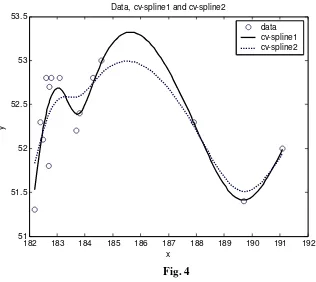
Data, test function and cv-spline

[image:6.595.164.439.84.343.2]

test function cv-spline data

Fig. 3

We observe that, for a too large value of

λ

, the estimated curve is not so close to data but is more smooth than real curve and for a too small value of

λ

, the estimated curve is not so smooth but is closer to data than the real curve is.

By contrast, the CV-value of

λ

gives us an optimal estimator. In this case, the estimated curve is more like the real one, not too close to data and not too smooth. 4.An application to real data

We will consider the same data as in [2], namely the observed values for the gas productivity,

x

i and the feedstock flow,

y

i, during 15 days, in the cracking

process.

In that paper, the cubic smoothing spline was obtained also from CV method, but using the bootstrap method, for resampling. The optimal value for

λ

was 0,11.

For the same data, we apply our algorihtm presented here and we obtain the optimal value for

λ

,

λ

_CV

=

0

,

0102

.

182 183 184 185 186 187 188 189 190 191 192 51

51.5 52 52.5 53 53.5

Data, cv-spline1 and cv-spline2

x

y

[image:7.595.128.444.90.372.2]

data cv-spline1 cv-spline2

Fig. 4

It can be observed that our curve is more closely to data and 0,11-curve is more smooth.

But obviuosly, at this point, we cannot say that the estimator presented here is better than estimator from [2], but just that the estimator presented here is more close to data. For choosing one method, inspite the other, we must know more about the real process.

For example, if one knows that he is interested more in goodness of fit than in smoothness, he will choose the estimator with

λ

=

0

,

0102

.

As a conclusion, if we know something prior about the “quantum” of the goodness of fit, or about the “quantum” of the smoothness, we can impose that the related term from (1) does not exceed an assumed tolerance.

References

1.Eubank R. L. - Nonparametric Regression and Spline Smoothing-Second Edition, Marcel Dekker, Inc., New York , Basel, 1999

3.Micula G.-Funcţii spline şi aplicaţii, Ed. Tehnică, Bucureşti, 1978

4.Micula G., Micula S.-Handbook of Splines, Kluwer Academic Publishers, Dordrecht/Boston/London, 1999

5.Stapleton J.H.- Linear Statistical Models. A Willey-Interscience Publications, Series in Probability and Statistics, New York, 1995

6.Wahba G.-Spline Models for Observational Data, SIAM Publications, Philadelphia, 1990

Author: