Chapter Sixteen
Chapter Outline
1) Overview
2) Relationship Among Techniques 2) One-Way Analysis of Variance
3) Statistics Associated with One-Way Analysis of Variance 4) Conducting One-Way Analysis of Variance
i. Identification of Dependent & Independent
Variables
ii. Decomposition of the Total Variation iii. Measurement of Effects
iv. Significance Testing
Chapter Outline
5) Illustrative Data
6) Illustrative Applications of One-Way Analysis of
Variance
7) Assumptions in Analysis of Variance
8) N-Way Analysis of Variance
9) Analysis of Covariance
10) Issues in Interpretation
i. Interactions
ii. Relative Importance of Factors iii. Multiple Comparisons
Chapter Outline
12) Nonmetric Analysis of Variance 13) Multivariate Analysis of Variance
14) Internet and Computer Applications 15) Focus on Burke
16) Summary
Relationship Among Techniques
Analysis of variance (ANOVA) is used as a
test of means for two or more populations.
The null hypothesis, typically, is that all means are equal.
Analysis of variance must have a dependent
variable that is metric (measured using an interval or ratio scale).
There must also be one or more independent
variables that are all categorical (nonmetric). Categorical independent variables are also
Relationship Among Techniques
A particular combination of factor levels, or
categories, is called a treatment.
One-way analysis of variance involves only one
categorical variable, or a single factor. In one-way analysis of variance, a treatment is the same as a factor level.
If two or more factors are involved, the analysis is
termed n-way analysis of variance.
If the set of independent variables consists of both
categorical and metric variables, the technique is called analysis of covariance (ANCOVA). In this case, the categorical independent variables are still referred to as factors, whereas the metric-independent variables are referred to as
16-7
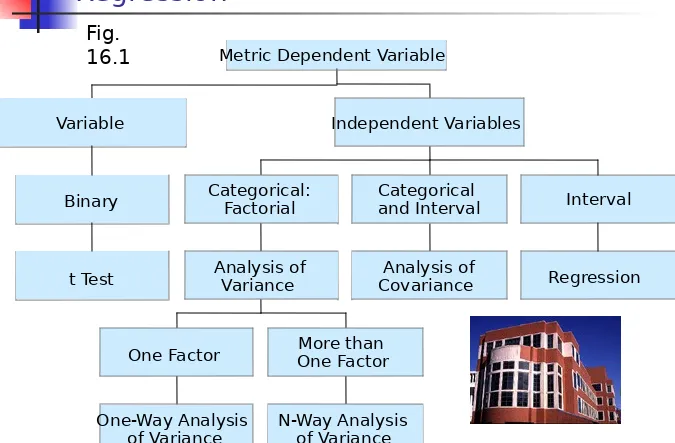
Relationship Amongst Test, Analysis of
Variance, Analysis of Covariance, &
Regression
Fig. 16.1
One Independent One or More Metric Dependent Variable
[image:7.720.23.698.62.505.2]One-way Analysis of Variance
Marketing researchers are often interested in
examining the differences in the mean values of the dependent variable for several categories of a single independent variable or factor. For
example:
Do the various segments differ in terms of their
volume of product consumption?
Do the brand evaluations of groups exposed to
different commercials vary?
What is the effect of consumers' familiarity with
16-9
Statistics Associated with One-way
Analysis of Variance
eta2 ( 2). The strength of the effects of X
(independent variable or factor) on Y (dependent
variable) is measured by eta2 ( 2). The value of
2 varies between 0 and 1.
F statistic. The null hypothesis that the
category means are equal in the population is
tested by an F statistic based on the ratio of
mean square related to X and mean square
related to error.
Mean square. This is the sum of squares
divided by the appropriate degrees of freedom.
16-10
Statistics Associated with One-way
Analysis of Variance
SSbetween. Also denoted as SSx, this is the
variation in Y related to the variation in the
means of the categories of X. This represents variation between the categories of X, or the portion of the sum of squares in Y related to X.
SSwithin. Also referred to as SSerror, this is the
variation in Y due to the variation within each of the categories of X. This variation is not accounted for by X.
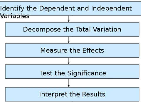
Conducting One-way ANOVA
Interpret the Results
Identify the Dependent and Independent Variables
Decompose the Total Variation
Measure the Effects
[image:11.720.139.619.134.483.2]Test the Significance
16-12
Conducting One-way Analysis of Variance
Decompose the Total Variation
The total variation in Y, denoted by SSy, can be
decomposed into two components:
SSy = SSbetween + SSwithin
where the subscripts between and within refer to the categories of X. SSbetween is the variation in Y
related to the variation in the means of the
categories of X. For this reason, SSbetween is also
denoted as SSx. SSwithin is the variation in Y
related to the variation within each category of X.
SSwithin is not accounted for by X. Therefore it is
16-13
The total variation in Y may be decomposed as:
SSy = SSx + SSerror
where
Yi = individual observation
j = mean for category j
= mean over the whole sample, or grand mean
Yij = i th observation in the j th category
Conducting One-way Analysis of Variance
Decompose the Total Variation
SSy= (YiY 2) i=1
N
SSx=
n (Y jY )2 j=1c
SSerror=
i n
(Y ijY j)2
j c
16-14
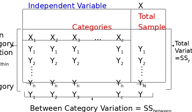
Decomposition of the Total Variation:
One-way ANOVA
Independent Variable X
Total
Categories Sample
X1 X2 X3 … Xc
Y1 Y1 Y1 Y1 Y1
Y2 Y2 Y2 Y2 Y2
: :
: :
Yn Yn Yn Yn YN
Y1 Y2 Y3 Yc Y
Within Category Variation =SSwithin
Between Category Variation = SSbetween
Total
Variation =SSy
[image:14.720.71.699.115.482.2]Category Mean
Conducting One-way Analysis of Variance
In analysis of variance, we estimate two measures of variation: within groups (SSwithin) and between
groups (SSbetween). Thus, by comparing the Y
variance estimates based on between-group and within-group variation, we can test the null
hypothesis.
Measure the Effects
The strength of the effects of X on Y are measured as follows:
2 = SSx/SSy = (SSy - SSerror)/SSy
The value of 2 varies between 0 and 1.
16-16
Conducting One-way Analysis of Variance
Test Significance
In one-way analysis of variance, the interest lies in testing the null hypothesis that the category means are equal in the population.
H0: µ1 = µ2 = µ3 = ... = µc
Under the null hypothesis, SSx and SSerror come from the same
source of variation. In other words, the estimate of the population variance of Y,
= SSx/(c - 1)
= Mean square due to X
= MSx
or
= SSerror/(N - c)
= Mean square due to error = MSerror
S
y2
S
y16-17
Conducting One-way Analysis of Variance
Test Significance
The null hypothesis may be tested by the F
statistic
based on the ratio between these two estimates:
This statistic follows the F distribution, with (c - 1) and
(N - c) degrees of freedom (df).
F = SSx/(c 1)
16-18
Conducting One-way Analysis of Variance
Interpret the Results
If the null hypothesis of equal category means
is not rejected, then the independent variable does not have a significant effect on the
dependent variable.
On the other hand, if the null hypothesis is
rejected, then the effect of the independent variable is significant.
A comparison of the category mean values will
16-19
Illustrative Applications of One-way
Analysis of Variance
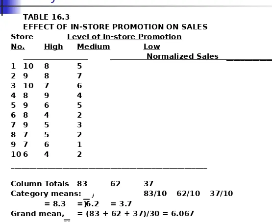
We illustrate the concepts discussed in this
chapter using the data presented in Table 16.2.
The department store is attempting to determine the effect of in-store promotion (X) on sales (Y). For the purpose of illustrating hand calculations, the data of Table 16.2 are transformed in Table 16.3 to show the store sales (Yij) for each level of
promotion.
The null hypothesis is that the category means are equal:
16-20
Effect of Promotion and Clientele on
Sales
Store Number Coupon Level In-Store Prom otion Sales Clientel Rating
1 1.00 1.00 10.00 9.00
2 1.00 1.00 9.00 10.00
3 1.00 1.00 10.00 8.00
4 1.00 1.00 8.00 4.00
5 1.00 1.00 9.00 6.00
6 1.00 2.00 8.00 8.00
7 1.00 2.00 8.00 4.00
8 1.00 2.00 7.00 10.00
9 1.00 2.00 9.00 6.00
10 1.00 2.00 6.00 9.00
11 1.00 3.00 5.00 8.00
12 1.00 3.00 7.00 9.00
13 1.00 3.00 6.00 6.00
14 1.00 3.00 4.00 10.00
15 1.00 3.00 5.00 4.00
16 2.00 1.00 8.00 10.00
17 2.00 1.00 9.00 6.00
18 2.00 1.00 7.00 8.00
19 2.00 1.00 7.00 4.00
20 2.00 1.00 6.00 9.00
21 2.00 2.00 4.00 6.00
22 2.00 2.00 5.00 8.00
23 2.00 2.00 5.00 10.00
24 2.00 2.00 6.00 4.00
25 2.00 2.00 4.00 9.00
26 2.00 3.00 2.00 4.00
27 2.00 3.00 3.00 6.00
28 2.00 3.00 2.00 10.00
29 2.00 3.00 1.00 9.00
30 2.00 3.00 2.00 8.00
16-21
[image:21.720.57.612.63.516.2]Illustrative Applications of One-way
Analysis of Variance
TABLE 16.3
EFFECT OF IN-STORE PROMOTION ON SALES Store Level of In-store Promotion
No. High Medium Low
Normalized Sales _________________
1 10 8 5
2 9 8 7
3 10 7 6
4 8 9 4
5 9 6 5
6 8 4 2
7 9 5 3
8 7 5 2
9 7 6 1
10 6 4 2
_____________________________________________________
Column Totals 83 62 37
Category means: j 83/10 62/10 37/10
= 8.3 = 6.2 = 3.7
Grand mean, = (83 + 62 + 37)/30 = 6.067
Y
16-22
To test the null hypothesis, the various sums of squares are computed as follows:
SSy = (10-6.067)2 + (9-6.067)2 + (10-6.067)2 + (8-6.067)2 +
(9-6.067)2
+ (8-6.067)2 + (9-6.067)2 + (7-6.067)2 + (7-6.067)2 + (6-6.067)2
+ (8-6.067)2 + (8-6.067)2 + (7-6.067)2 + (9-6.067)2 + (6-6.067)2
(4-6.067)2 + (5-6.067)2 + (5-6.067)2 + (6-6.067)2 + (4-6.067)2
+ (5-6.067)2 + (7-6.067)2 + (6-6.067)2 + (4-6.067)2 + (5-6.067)2
+ (2-6.067)2 + (3-6.067)2 + (2-6.067)2 + (1-6.067)2 + (2-6.067)2
=(3.933)2 + (2.933)2 + (3.933)2 + (1.933)2 + (2.933)2
+ (1.933)2 + (2.933)2 + (0.933)2 + (0.933)2 + (-0.067)2
+ (1.933)2 + (1.933)2 + (0.933)2 + (2.933)2 + (-0.067)2
(-2.067)2 + (-1.067)2 + (-1.067)2 + (-0.067)2 + (-2.067)2
+ (-1.067)2 + (0.9333)2 + (-0.067)2 + (-2.067)2 + (-1.067)2
+ (-4.067)2 + (-3.067)2 + (-4.067)2 + (-5.067)2 + (-4.067)2
= 185.867
16-23
SSx = 10(8.3-6.067)2 + 10(6.2-6.067)2 + 10(3.7-6.067)2
= 10(2.233)2 + 10(0.133)2 + 10(-2.367)2
= 106.067
SSerror = (10-8.3)2 + (9-8.3)2 + (10-8.3)2 + (8-8.3)2 + (9-8.3)2
+ (8-8.3)2 + (9-8.3)2 + (7-8.3)2 + (7-8.3)2 + (6-8.3)2
+ (8-6.2)2 + (8-6.2)2 + (7-6.2)2 + (9-6.2)2 + (6-6.2)2
+ (4-6.2)2 + (5-6.2)2 + (5-6.2)2 + (6-6.2)2 + (4-6.2)2
+ (5-3.7)2 + (7-3.7)2 + (6-3.7)2 + (4-3.7)2 + (5-3.7)2
+ (2-3.7)2 + (3-3.7)2 + (2-3.7)2 + (1-3.7)2 + (2-3.7)2
= (1.7)2 + (0.7)2 + (1.7)2 + (-0.3)2 + (0.7)2
+ (-0.3)2 + (0.7)2 + (-1.3)2 + (-1.3)2 + (-2.3)2
+ (1.8)2 + (1.8)2 + (0.8)2 + (2.8)2 + (-0.2)2
+ (-2.2)2 + (-1.2)2 + (-1.2)2 + (-0.2)2 + (-2.2)2
+ (1.3)2 + (3.3)2 + (2.3)2 + (0.3)2 + (1.3)2
+ (-1.7)2 + (-0.7)2 + (-1.7)2 + (-2.7)2 + (-1.7)2
= 79.80
16-24
It can be verified that
SSy = SSx + SSerror
as follows:
185.867 = 106.067 +79.80
The strength of the effects of X on Y are measured as follows: 2 = SSx/SSy
= 106.067/185.867 = 0.571
In other words, 57.1% of the variation in sales (Y) is accounted for by in-store promotion (X), indicating a modest effect. The null hypothesis may now be tested.
= 17.944
F = SSx/(c 1)
SSerror/(N c) = MSMSerrorX
F= 106.067/(31) 79.800/(303)
16-25
From Table 5 in the Statistical Appendix we see
that for 2 and 27 degrees of freedom, the
critical value of F is 3.35 for . Because the calculated value of F is greater than the critical value, we reject the null hypothesis.
We now illustrate the analysis of variance
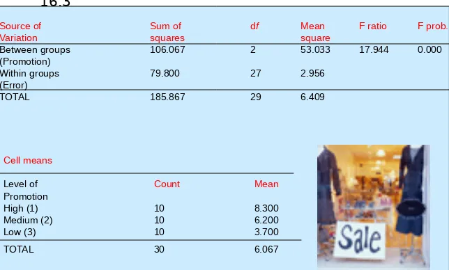
procedure using a computer program. The results of conducting the same analysis by computer are presented in Table 16.4.
= 0.05
16-26
One-Way ANOVA:
Effect of In-store Promotion on Store Sales
Table 16.3
Cell means
Level of Count Mean
Promotion
High (1) 10 8.300
Medium (2) 10 6.200
Low (3) 10 3.700
TOTAL 30 6.067
Source of Sum of df Mean F ratio F prob.
Variation squares square
Between groups 106.067 2 53.033 17.944 0.000
(Promotion)
Within groups 79.800 27 2.956
(Error)
[image:26.720.46.690.117.505.2]16-27
Assumptions in Analysis of
Variance
The salient assumptions in analysis of variance can be summarized as follows.
1. Ordinarily, the categories of the independent
variable are assumed to be fixed. Inferences are made only to the specific categories considered. This is referred to as the fixed-effects model.
2. The error term is normally distributed, with a
zero mean and a constant variance. The error is not related to any of the categories of X.
3. The error terms are uncorrelated. If the error
N-way Analysis of Variance
In marketing research, one is often concerned with the effect of more than one factor simultaneously. For example:
How do advertising levels (high, medium, and low)
interact with price levels (high, medium, and low) to influence a brand's sale?
Do educational levels (less than high school, high
school
graduate, some college, and college graduate) and age (less than 35, 35-55, more than 55) affect
consumption of a brand?
What is the effect of consumers' familiarity with a
N-way Analysis of Variance
Consider the simple case of two factors X1 and X2 having
categories c1 and c2. The total variation in this case is
partitioned as follows:
SStotal = SS due to X1 + SS due to X2 + SS due to interaction of X1
and X2 + SSwithin
or
The strength of the joint effect of two factors, called the overall effect, or multiple 2, is measured as follows:
multiple 2 =
SSy = SSx1 + SSx2 + SSx1x2 + SSerror
N-way Analysis of Variance
The significance of the overall effect may be tested by an F
test, as follows
where
dfn = degrees of freedom for the numerator
= (c1 - 1) + (c2 - 1) + (c1 - 1) (c2 - 1)
= c1c2 - 1
dfd = degrees of freedom for the denominator
= N - c1c2
MS = mean square
F = (SSx1 + SSx2 + SSx1x2)/dfn
SSerror/dfd
= SSx1,x2,x1x2/ dfn SSerror/dfd
= MSx1,x2,x1x2
N-way Analysis of Variance
If the overall effect is significant, the next step is to
examine the significance of the interaction effect. Under the null hypothesis of no interaction, the
appropriate F test is:
where
dfn = (c1 - 1) (c2 - 1)
dfd = N - c1c2
F = SSx1x2/dfn
SSerror/dfd
= MSx1x2
N-way Analysis of Variance
The significance of the main effect of each factor
may be tested as follows for X1:
where
dfn = c1 - 1
dfd = N - c1c2
F = SSx1/dfn
SSerror/dfd
= MSx1
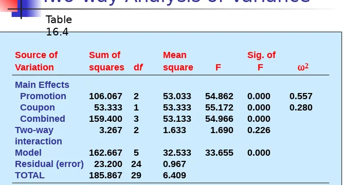
Two-way Analysis of Variance
Source of Sum of Mean Sig. of
Variation squares df square F F
Main Effects
Promotion 106.067 2 53.033 54.862 0.000 0.557
Coupon 53.333 1 53.333 55.172 0.000 0.280
Combined 159.400 3 53.133 54.966 0.000
Two-way 3.267 2 1.633 1.690 0.226
interaction
Model 162.667 5 32.533 33.655 0.000
Residual (error) 23.200 24 0.967
TOTAL 185.867 29 6.409
2
[image:33.720.20.691.58.418.2]Two-way Analysis of Variance
Table 16.4 cont.
Cell Means
Promotion Coupon Count Mean High Yes 5 9.200 High No 5 7.400 Medium Yes 5 7.600 Medium No 5 4.800 Low Yes 5 5.400 Low No 5 2.000
TOTAL 30
Factor Level Means
Analysis of Covariance
When examining the differences in the mean values of the dependent variable related to the effect of the
controlled independent variables, it is often necessary to take into account the influence of uncontrolled
independent variables. For example:
In determining how different groups exposed to different
commercials evaluate a brand, it may be necessary to control for prior knowledge.
In determining how different price levels will affect a
household's cereal consumption, it may be essential to take household size into account. We again use the data of Table 16.2 to illustrate analysis of covariance.
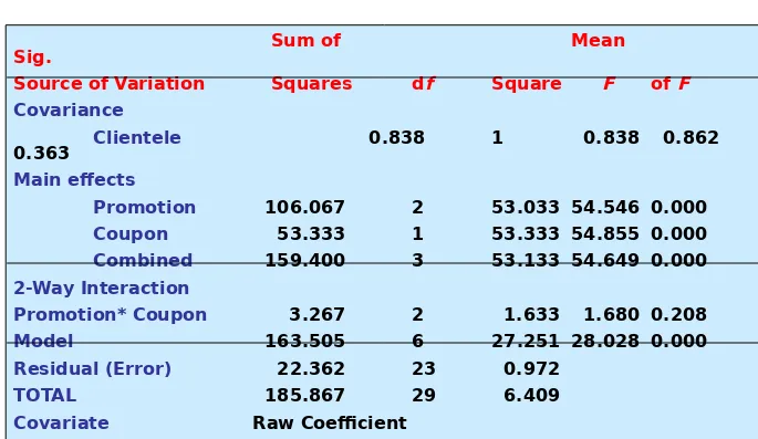
Suppose that we wanted to determine the effect of
in-store promotion and couponing on sales while
Analysis of Covariance
Sum of Mean
Sig.
Source of Variation Squares df Square F of F
Covariance
Clientele 0.838 1 0.838 0.862
0.363
Main effects
Promotion 106.067 2 53.033 54.546 0.000
Coupon 53.333 1 53.333 54.855 0.000
Combined 159.400 3 53.133 54.649 0.000
2-Way Interaction
Promotion* Coupon 3.267 2 1.633 1.680 0.208
Model 163.505 6 27.251 28.028 0.000
Residual (Error) 22.362 23 0.972
TOTAL 185.867 29 6.409
Covariate Raw Coefficient
[image:36.720.18.703.128.525.2]Clientele -0.078
Issues in Interpretation
Important issues involved in the interpretation of ANOVA results include interactions, relative importance of factors, and multiple comparisons.
Interactions
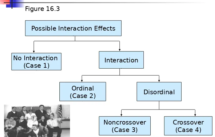
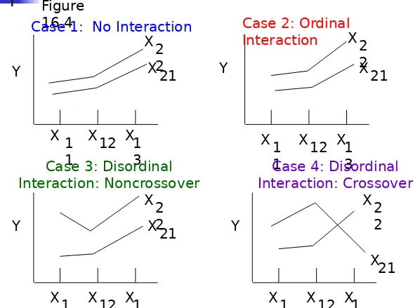
The different interactions that can arise when
conducting ANOVA on two or more factors are shown in Figure 16.3.
Relative Importance of Factors
Experimental designs are usually balanced, in that each
cell contains the same number of respondents. This results in an orthogonal design in which the factors are uncorrelated. Hence, it is possible to determine
16-38
A Classification of Interaction
Effects
Noncrossover (Case 3)
Crossover (Case 4) Possible Interaction Effects
No Interaction
(Case 1) Interaction
Ordinal
[image:38.720.23.711.67.506.2]Patterns of Interaction
Figure 16.4
Y
X 1 X X 1
12 1 3
Case 1: No Interaction
X 2 2 X 21
X1 X X 1 12 1 3 X2 2 X 21 Y
Case 2: Ordinal Interaction
Y
X1 X X 1 12 1 3 X 2 2 X 21
Case 3: Disordinal Interaction: Noncrossover
Y
X1 X X 1 12 1 3 X2 2 X21
Issues in Interpretation
The most commonly used measure in ANOVA is omega
squared, . This measure indicates what proportion of the variation in the dependent variable is related to a particular independent variable or factor. The relative contribution of a factor X is calculated as follows:
Normally, is interpreted only for statistically significant
effects. In Table 16.5, associated with the level of in-store promotion is calculated as follows:
= 0.557
x2 = SSx (dfx x MSerror)
SStotal + MSerror
p2 = 106.067 (2 x 0.967) 185.867 + 0.967
= 104.133 186.834
2
2
Issues in Interpretation
Note, in Table 16.5, that
SStotal = 106.067 + 53.333 + 3.267 + 23.2
= 185.867
Likewise, the associated with couponing is:
= 0.280
As a guide to interpreting , a large experimental effect produces an index of 0.15 or greater, a medium effect produces an index of around 0.06, and a small effect
produces an index of 0.01. In Table 16.5, while the effect of promotion and couponing are both large, the effect of promotion is much larger.
2
c2 = 53.333 (1 x 0.967)
185.867 + 0.967
16-42
Issues in Interpretation
Multiple Comparisons
If the null hypothesis of equal means is
rejected, we can only conclude that not all of the group means are equal. We may wish to examine differences among specific means. This can be done by specifying appropriate
contrasts, or comparisons used to determine
which of the means are statistically different.
A priori contrasts are determined before
conducting the analysis, based on the
researcher's theoretical framework. Generally, a priori contrasts are used in lieu of the ANOVA
16-43
Issues in Interpretation
Multiple Comparisons
A posteriori contrasts are made after the
analysis. These are generally multiple
comparison tests. They enable the researcher to construct generalized confidence intervals
that can be used to make pairwise comparisons of all treatment means. These tests, listed in order of decreasing power, include least
significant difference, Duncan's multiple range test, Student-Newman-Keuls, Tukey's alternate procedure, honestly significant difference,
modified least significant difference, and
Repeated Measures ANOVA
One way of controlling the differences between subjects is by observing each subject under
each experimental condition (see Table 16.7). Since repeated measurements are obtained from each respondent, this design is referred to as within-subjects design or repeated
measures analysis of variance. Repeated
16-45
Decomposition of the Total Variation:
Repeated Measures ANOVA
Independent Variable X
Subject Categories Total
No. Sample
X1 X2 X3 … Xc
1 Y11 Y12 Y13 Y1c Y1
2 Y21 Y22 Y23 Y2c Y2
: :
: :
n Yn1 Yn2 Yn3 Ync YN
Y1 Y2 Y3 Yc Y
Between People Variation =SSbetween people Total Variation =SSy
Within People Category Variation = SSwithin people
[image:45.720.39.691.127.505.2]Category Mean
Repeated Measures ANOVA
In the case of a single factor with repeated measures, the total variation, with nc - 1 degrees of freedom, may be split into between-people variation and within-people variation.
SStotal = SSbetween people + SSwithin people
The between-people variation, which is related to the differences between the means of people, has n - 1 degrees of freedom. The within-people variation has
n (c - 1) degrees of freedom. The within-people variation may, in turn, be divided into two different sources of
variation. One source is related to the differences between treatment means, and the second consists of residual or error variation. The degrees of freedom corresponding to the treatment variation are c - 1, and those corresponding to residual variation are
Repeated Measures ANOVA
Thus,
SSwithin people = SSx + SSerror
A test of the null hypothesis of equal means may now be constructed in the usual way:
So far we have assumed that the dependent variable is measured on an interval or ratio scale. If the dependent variable is nonmetric, however, a different procedure should be used.
F = SSx/(c 1)
Nonmetric Analysis of Variance
Nonmetric analysis of variance
examines the difference in the central
tendencies of more than two groups when
the dependent variable is measured on an
ordinal scale.
One such procedure is the
k
-sample
median test
. As its name implies, this is
Nonmetric Analysis of Variance
A more powerful test is the Kruskal-Wallis one way
analysis of variance. This is an extension of the
Mann-Whitney test (Chapter 15). This test also examines the difference in medians. All cases from the k groups are ordered in a single ranking. If the k populations are the same, the groups should be similar in terms of ranks within each group. The rank sum is calculated for each group. From these, the Kruskal-Wallis H statistic, which has a chi-square distribution, is computed.
The Kruskal-Wallis test is more powerful than the k
-sample median test as it uses the rank value of each case, not merely its location relative to the median.
However, if there are a large number of tied rankings in the data, the k-sample median test may be a better
Multivariate Analysis of Variance
Multivariate analysis of variance
(MANOVA) is similar to analysis of variance
(ANOVA), except that instead of one metric dependent variable, we have two or more.
In MANOVA, the null hypothesis is that the
vectors of means on multiple dependent variables are equal across groups.
Multivariate analysis of variance is appropriate
SPSS Windows
One-way ANOVA can be efficiently performed using the program COMPARE MEANS and then One-way ANOVA. To select this procedure
using SPSS for Windows click:
Analyze>Compare Means>One-Way ANOVA …
N-way analysis of variance and analysis of
covariance can be performed using GENERAL LINEAR MODEL. To select this procedure using SPSS for Windows click:
