CONSERVATION AND DECAY IN PHYSICAL
MODELLING
Frits P.H. van Beckum
Abstract. Mathematical modeling of physical phenomena is mainly governed by
conservation laws (mass, momentum, heat, etc) and by principles like ”Physics will always decay to equilibrium, will strive for minimal energy”, etc. Therefore, in the resulting mathematical model, e.g. a system of ordinary or partial differential equations, it makes sense to recognize and distinguish the terms and structures that are related to conservation from those that are responsible for decay. Examples are mainly taken in the field of heat transfer and wave propagation. Here, with ”terms” we mean: the spatial derivatives of first and higher order and as examples of ”structure” we first have the well-known Hamiltonian structure [1, 2](both in ordinary and in partial differential equations) which guarantees conservation, but we will also see its extension to models where decay plays a role. These insights can be of profit for numerical calculation [3]. In general purpose algorithms the conservation properties are generally lost, due to numerical errors. However, if we construct an algorithm following the special structure of the equations, then it will inherit the conservation properties. One of the consequences is e.g. that in models with decay, we can be sure that the decay that we calculate is not due to numerics, but is exactly representing the physics that we have modeled in the equations.
1. INTRODUCTION
Mathematicians will not aiming at a full definition agree that mathe-matics can be seen as a quantitative science about abstract objects and their properties. In university courses and textbooks mathematics may mainly
Received 28-11-2012, Accepted 24-12-2012.
2010 Mathematics Subject Classification: 35-XX, 65P10, 91B72.
Key words and Phrases: Hamiltonian Structure, Riemann Invariants, Partial Differential Equa-tions.
seem a science of definition theorem proof , while in high school the mem-orizing of formulas and the application of tricks may sometimes dominate the perception rather than the understanding of methods and results.
Among these and more points of view, an important way of looking at mathematics is given by: a science of structures. This of course includes geometrical constructions but also algebraic structures like rings and mod-ules, analytic structures like Banach spaces, and many others in discrete mathematics, probability, etc. In this paper we restrict to structures in par-tial differenpar-tial equations, in particular the basic wave equations that are used in fluid dynamics and hydraulic engineering, and we give three exam-ples of what these structures tell about the behavior of the solution, the propagation of physical quantities, and their conservation or decay.
The subjects collected here have been studied in cooperation projects between Indonesia and the Netherlands, which started in 1990 and are still going on. It is with great pleasure that I review some of them here in Medan.
2. RECOGNIZE THE EFFECT OF SPATIAL DERIVATIVES
This chapter will be about waves of the formu(x, t), function of time tand of one spatial variable x. Specifically, we will consider waves that initially are harmonic, i.e. have a pure sinusoidal form, and we will consider how they deform as a solution of a linear partial differential equation of a specific form: first order in time and any finite (but still low) order inx. At the end we will consider one nonlinear case, involving the most frequently occurring nonlinear termuux.
Translation equation
The simplest partial differential equation one can think of is
ut+cux = 0 (1)
where subscripts denote derivation with respect totandxrespectively. The constantccould even be scaled away, but we leave it in, mainly to allow for tracing the physical dimensions, if desirable.
Let us consider a wave that initially, i.e. att= 0, has a sinusoidal pro-file: sin(kx), cos(kx), or a linear combination of both, which we conveniently represent in the complex notation
wherek is any real number, called the wave number, then
u(x, t) =eikxe−ikct =eik(x−ct) (3)
so at every moment the wave is a translation of the initial shape: the wave is running to the right with velocity c. Alternatively, when looking at the wave at a fixed position x, we see a harmonic (sinusoidal) motion in time with one fixed frequencyω:
ω=kc. (4)
Therefore the wave is calledmonochromatic, a term from the theory of light waves, where one frequency selects one specific colour.
Remark. A systematic way to find solutions is to try a separated solution, i.e. a function of x only, multiplied with a function of t only: u(x, t) = f(x)g(t). The initial condition requiresf to be: f(x) = eikx, and from the
differential equation we find that g takes the form eikct. Or, as a further shortcut: once we are convinced that the time-functiong is an exponential, we adopt the Ansatz
u(x, t) =eikx−iωt (5)
and by substituting in the differential equation we find how ω relates to k.
Dissipation
If we add a second order derivative to the differential equation:
ut+cux=νuxx (6)
and apply the Ansatz (5), we find −iω=−ick−k2ν, so the solution is
u(x, t) =eik(x−ct)e−k2νt. (7)
Dispersion
If we extend the translation equation (1) with a third order derivative:
ut+cux+εuxxx= 0 (8)
the same procedure leads to
ω=ck−εk3 (9)
from which we find the solution:
u(x, t) =u(x, t) =eik(x−(c−εk2)t). (10)
Comparing with (3), we see the solution is again a harmonic, monochromatic wave (no damping), however with a modified velocity: c−εk2. Note that this modification of velocity is depending onk: for positiveε(as is occurring in waves), the speed decreases with wave length: small wave lengths run slower than long ones.
Remark 1. Relation (9) is called the dispersion relation. In fact, already (4) was a dispersion relation too. For equation (6) the dispersion relation will have imaginary terms, denoting that there is dissipation.
Remark 2. Another dispersive term met in differential equations is the mixed derivative uxxt, which is typical for Boussinesq wave models [4, 5].
The equation
ut+cux+εuxxt= 0 (11)
has the dispersion relation
ω=c k
a+εk2 (12)
Forkbeing small which is an assumption in Boussinesq models this formula agrees with (9); but the nice property of (12) is that for larger wave num-ber k the wave velocity is still positive (and goes to zero), while from (9) velocities become negative which is unphysical.
Zeroth order derivative
In this overview of what the effect is of spatial derivatives on wave behavior, we can even consider a term with the 0th derivative, that is the
function itself. Such a term occurs e.g. as the friction term in the partial differential equation
where the friction factor f is positive and in the simplest case a constant. Then a solution is
u(x, t) =e−f teik(x−ct)
as everyone can easily verify. The effect is exponential uniform damping, i.e. a damping that is independent of the wave numberk.
We remember that the second derivative also gives damping of am-plitude, but in a selective way: depending on the wave number. Similar difference is found between the third and first derivative, but then with respect to the wave speed.
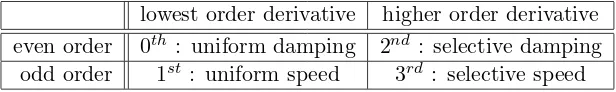
We give a summarizing table 1
Table 1: What effect spatial derivatives in linear equations have
lowest order derivative higher order derivative even order 0th : uniform damping 2nd : selective damping
odd order 1st : uniform speed 3rd : selective speed
Nonlinear steepening
Nonlinearity can, in principle, occur in any term of any equation. But if we say: the nonlinear term, we always mean a term likeuux, the nonlinear
advection term. Let us consider the simple nonlinear equation
ut+uux= 0 (13)
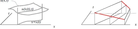
Compared with equation (1) wherecis the wave velocity, we now see that u itself is the velocity. Therefore, higher values ofuwill run faster than lower ones, wave crests run faster than troughs. As a consequence, leading slopes of a wave will get steeper, and trailing slopes will stretch [6]. The wave will turn over, and eventually break, like we can observe in the surf zone, as depicted in figure 1. (Actually, the effect is depending on water depth: the smaller the depth, the stronger the steepening.)
Let us give a mathematical support of this verbal description of the steepening phenomenon. Take a curve x = x(t) in the x, t-plane. Then, considered along this curve, the solution u(x, t) becomes a function of t only: u = u(x(t), t). (See figure 3, left.) The full time-derivative of this function is:
d
dtu(x(t), t) = ∂u ∂x
dx dt +
∂u
∂t =ut+ dx
Figure 1: The effect is depending on water depth
Now in view of (13) we can say: if dx
dt =ueverywhere along this curve, then
(14) is 0, which implies that u(x(t), t) is a constant along the curve. But as uis the slope of the curve, this curve must be a straight line, its slope being given by the value ofu(x(t), t) att= 0 , that is: the initial data at the point where the line intersects thex-axis. So from every point on the initial line, the x-axis, we can see how the value of u propagates into thex, t-plane, as illustrated in next figure 3 (right), the higher values of u running faster, the lower values running slower, and thus creating a more steeper wave front.
Figure 2: The value ofu propagates into thex, t-plane
Combinations of terms
Dispersion and dissipation have been introduced as linear effects, act-ing on a mono-chromatic wave. As a general wave can be represented by a Fourier series or Fourier integral, through the principle of superposition we can imagine the result for any wave profile. This is no longer true in nonlinear equations like (13). In fact, starting with a monochromatic wave (2), the nonlinear term will become eikxikeikx = ikei2kx, so it generates a
and dissipation are counteracting to nonlinear steepening in this sense. The two model equations for this type of counteraction are equation
ut+uux=νuxx, theBurgersequation (15)
combining nonlinear steepening with dissipation, and
ut+uux+εuxxx, theKortewegdeVriesequation (16)
where nonlinear steepening is combined with dispersion. There is a world of literature on these equations. We will no further go into the interaction of two terms, as the aim of this chapter was to recognize the effect of single terms only.
3. SHALLOW WATER EQUATION
Continuity equation
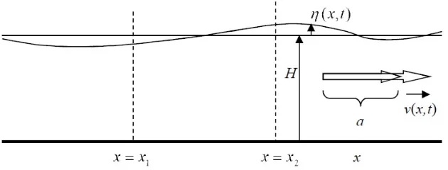
In this one-dimensional channel consider a volumeV bounded by two vertical cross sections, chosen at two arbitrary positionsx=x1 and x=x2
respectively, as depicted in figure ??. The total mass of water within this volume is the integral of the density over V:
M =
We will make use of the conservation of mass in the volume V while the cross sections bounding V are moving along with the flow. Since the water velocity, u =u(x, t), is not dependent on z, it may help our imagination if we would think of the volume V as being bounded by two vertical sheets of plastic (impermeable and light enough not to influence the momentum of the flow): they will keep vertical and keep being the bounds of the water volume V, while their positions x1 and x2 are moving with time: x1 =x1(t) and
x2=x2(t). The conservation of mass withinV is mathematically expressed
by stating that during the motion the value ofM is independent of time, so in view of (17):
0 =dtM =dt
Z x2(t)
x1(t)
h(x, t)dx (18)
Note thattis not only in the integrandh(x, t) but also in the integral bounds; so when performing the differentiation with respect to t we get (Leibniz rule that you learned in second years Calculus, where you always wondered if such a complicated expression would ever occur in practice!) :
0 =
dt is the speed of the first plastic sheet, which equals the speed of
the wateru(x, t) atx=x1(t); similar forx2 . So the last two terms of (19)
can jointly be written as an integral again:
h(x, t)|x=x2
Combined with the first term of (19) we have:
Z x2
x1
Remembering that x1 and x2 are chosen arbitrarily, we can conclude that
the integrand must be zero for all x :
∂th(x, t) +∂x{h(x, t)u(x, t)}= 0 (22)
This equation is called the continuity equation, or the mass balance, or the conservation of mass.
Continuity equation
For the same section [x1, x2] of our channel we consider the total
mo-mentum contained within the volumeV. In fact we restrict to the horizontal component. The horizontal momentum of a unit volume at position (x, z, t) is ρu(x, t), so the total momentum contained within the section is the inte-gral over V:
M om(t) =
Z x2(t)
x1(t)
Z h(x,t)
0
ρu(x, t)dzdx=ρ
Z x2(t)
x1(t)
h(x, t)u(x, t)dx (23)
Now this total horizontal momentum will change with time due to forces acting on it. Neglecting internal and external frictions or excitations, we are left with the forces exerted by the hydrostatic pressure. These are calculated as follows. The hydrostatic pressure at a point (x, z) is equal to (suppressing the notation of the time variable): p(x, z) =ρg(h(x)−z), whereh(x)−zis the height of the water column above the point (x, z). Now pressure is the value of the force acting per unit area perpendicular on it; so at position z on a plastic sheet, ρg(h−z) is the force acting in horizontal direction on the sheet per unit area, and the total forceF on the sheet is the integral of the pressure:
F =F(x) =
Z h(x,t)
0
ρg(h(x)−z)dz = 1
2ρgh(x, t)
2 (24)
The force acting on the volumeV, i.e. on the sheetx=x1 by the
result of these two forces on V is:
Having found the net forceF we come to expressing the momentum balance. The net force F is equal to the increase per second of the total momentum Mom within the volumeV:
d
Now, like we already noticed after eq. (19), the factor dx2(t)
dt is the
speed at which the position x2 moves and that is by definition equal to
u(x2(t), t); and similar forx1; so the last two terms of (26) together give: and so, when equating (25) to (26), we get
−ρg
Here all terms concern the same integration: Rx2(t)
x1(t), so when shifting all terms to one side of the equation we can combine them into one integral which should be equal to zero; remembering that x1 and x2 are arbitrary,
This is the momentum equation. In combination with the continuity equa-tion (22) it can be further simplified as follows. Omitting the variables (x, t), we first repeat (22) and (29):
(22) : ∂th+∂x(hu) = 0 (30)
(29) : ∂t(hu) +∂x(hu2) +gh∂xh= 0 ‘ (31)
and we expand the latter as follows:
h∂tu+u∂th+u∂x(hu) +hu∂xu+gh∂xh= 0 (32)
Now the second and third term of this equation (32) are recognized as a multiple of (30) and so they vanish; then the remaining equation can be divided through byh, leading to:
∂tu+u∂xh+g∂xh= 0 (33)
Here we arrive at the standard form of the (one-dimensional) Shallow Water Equations:
(
∂th+u∂xh+h∂xu= 0
∂tu+u∂xu+g∂xh= 0
(34)
Note that both equations have the differential operator∂t+u∂x, which
is the time derivative observed when moving along with the flow. Mathe-matically it is a kind of directional derivative in the x, t-plane. In the next subsection however we will meet another interesting directional derivative.
4. RIEMANN INVARIANTS
Matrix-vector analysis will reveal the basic structure of the SWE (34). We will do this analysis on the linearized form, as this is already enough to show the essentials, while going into the nonlinear details might absorb too much of the readers attention. Therefore, we linearize the quantities h and u :
h(x, t) =H+η(x, t) (35)
where H is the constant water height of the fluid in steady flow, and η is the elevation measured from this equilibrium level; and:
Figure 3: The basic structure of the SWE
whereais the constant flow velocity of the river (for a non-flowing channel we have a= 0 ), and v is the flow velocity in excess of a. Like u, both a and v are supposed to be independent on the spatial coordinates y andz.
Substituting (35) and (36) into (34) and assuming that the new de-pendent variables η and v are small enough to neglect second order terms (that is: products and squares ofη andv and their derivatives), will lead to the linearized SWE in these new variables:
(
this matrix will be named: C. Eigenvaluesλfollow from
(a−λ)2=gH →λ±=a±c (39)
with
c≡pgH (40)
Eigenvector forλ+ from:
Note from (40) and (41) thatc has the physical dimension of velocity and τ has the physical dimension of time.
Writing the two eigenvectors in a 2×2 matrix T:
1 τ 1 −τ
, this T
satisfiesT C = ΛT, where Λ is the diagonal matrix containing the eigenval-ues. So when multiplying system (38) with this T from the left we get
Now it is important to note the difference with the original system (37). In the original (linear) SWE, each of the equations contains a mix of both partial derivatives of both η and v. However, in the newly derived form we do two typical observations. Let us look at (43). Firstly, it has only one differential operator, and this operator ∂t+ (a+c)∂x is a directional
derivative in the x, t-plane; it is the time derivative measured along a line (curve) x = x(t) that has direction dxdt = a+c. This curve is called a characteristic, and in this case where aand c are constants, characteristics are straight lines: x= (a+c)t+x0. And secondly, this differential operator
acts on one specific combination ofη(x, t) and v(x, t), namely the quantity η(x, t)+τ v(x, t). So, considered along a characteristic, the equation (43 top) is in fact an ordinary differential equation for one dependent variable. And in this case it is very easy to see the solution: η(x, t) +τ v(x, t) is conserved along a right-running characteristic. Similarly, from (43 bottom) we have: η(x, t)−τ v(x, t) is conserved along a left-running characteristic.
ACKNOWLEDGEMENT
The author, looking back on many years of fruitful work and frienship in Indonesia, is indebted to the organisers of this Simantap for inviting him to Medan to further share the insights that this work has produced.
References
[2] F.P.H. van Beckum. 1995. Hamiltonian-consistent discretisation of wave equations. Ph.D Thesis, Univ. of Twente, the Netherlands.
[3] F.P.H. van Beckum and E. van Groesen. 1987. Discretizations conserv-ing energy and other constants of the motion. In: Proc. First Intl. Conf. on Ind. And Appl. Math. (ICIAM), A.H¿ P. van der Burgh and R.M.M. Mattheij (Eds), 17-35.
[4] S.R. Pudjaprasetya. 1996. Evolution of waves above slightly varying bottom: a variational approach. Ph.D Thesis, Univ. of Twente, the Netherlands.
[5] Gert Klopman. 2010. Variational Boussinesq modelling of surface grav-ity waves over bathymetry. VPh.D Thesis, Univ. of Twente, the Nether-lands.
[6] S.R. Pudjaprasetya, E. Khatizah. 2012. Longshore Submerged Wave Breaker for Reflecting Beach, East Asian Journal on Applied Mathe-matics (EAJAM) Vol. 2, No. 1, pp. 47-58.
Frits P.H. van Beckum: Former lecturer in Applied Mathematics University of
Twente, the Netherlands