A graph-theoretical clustering method based on two rounds of minimum spanning trees

(1)

Contents lists available atScienceDirect

Pattern Recognition

journal homepage:w w w . e l s e v i e r . c o m / l o c a t e / p r

A graph-theoretical clustering method based on two rounds of minimum

spanning trees

Caiming Zhong

a,b,c

_{, Duoqian Miao}

a,b,∗

_{, Ruizhi Wang}

a,b

a_{Department of Computer Science and Technology, Tongji University, Shanghai 201804, PR China}

b_{Key Laboratory of Embedded System & Service Computing, Ministry of Education of China, Shanghai 201804, PR China} c_{College of Science and Technology, Ningbo University, Ningbo 315211, PR China}

A R T I C L E I N F O A B S T R A C T

Article history:

Received 22 January 2009

Received in revised form 19 July 2009 Accepted 24 July 2009

Keywords:

Graph-based clustering Well-separated cluster Touching cluster Two rounds of MST

Many clustering approaches have been proposed in the literature, but most of them are vulnerable to the different cluster sizes, shapes and densities. In this paper, we present a graph-theoretical clustering method which is robust to the difference. Based on the graph composed of two rounds of minimum spanning trees (MST), the proposed method (2-MSTClus) classifies cluster problems into two groups, i.e. separated cluster problems and touching cluster problems, and identifies the two groups of cluster prob-lems automatically. It contains two clustering algorithms which deal with separated clusters and touching clusters in two phases, respectively. In the first phase, two round minimum spanning trees are employed to construct a graph and detect separated clusters which cover distance separated and density separated clusters. In the second phase, touching clusters, which are subgroups produced in the first phase, can be partitioned by comparing cuts, respectively, on the two round minimum spanning trees. The proposed method is robust to the varied cluster sizes, shapes and densities, and can discover the number of clusters. Experimental results on synthetic and real datasets demonstrate the performance of the proposed method. © 2009 Elsevier Ltd. All rights reserved.

1. Introduction

The main goal of clustering is to partition a dataset into clusters in terms of its intrinsic structure, without resorting to any a priori knowledge such as the number of clusters, the distribution of the data elements, etc. Clustering is a powerful tool and has been studied and applied in many research areas, which include image segmen-tation[1,2], machine learning, data mining[3], and bioinformatics

[4,5]. Although many clustering methods have been proposed in the recent decades, there is no universal one that can deal with all cluster problems, since in the real world clusters may be of arbitrary shapes, varied densities and unbalanced sizes[6,7]. In addition, Kleinberg

[8]presented an impossibility theorem to indicate that it is difficult to develop a universal clustering scheme. However, in general, users have not any a priori knowledge on their datasets, which makes it a tough task for them to select suitable clustering methods. This is the dilemma of clustering.

∗_{Corresponding author at: Department of Computer Science and Technology,} Tongji University, Shanghai 201804, PR China. Tel.: +86 21 69589867.

E-mail addresses:charman_zhong@hotmail.com(C. Zhong),

miaoduoqian@163.com(D. Miao).

Two techniques have been proposed and studied to alleviate the dilemma partially, i.e. clustering ensemble[9–11]and multiobjec-tive clustering [12]. The basic idea of a clustering ensemble is to use different data representation, apply different clustering methods with varied parameters, collect multiple clustering results, and dis-cover a cluster with better quality[13]. Fred and Jain[13]proposed a co-association matrix to depict and combine the different cluster-ing results by explorcluster-ing the idea of evidence accumulation. Topchy et al.[10]proposed a probabilistic model of consensus with a finite mixture of multinomial distributions in a space of clusterings, and used the EM algorithm to find the combined partitions. Taking ad-vantage of correlation clustering[14], Gionis et al.[11]presented a clustering aggregation framework, which can find a new clustering that minimizes the total number of disagreements with all the given clusterings. Being different from a clustering ensemble which is lim-ited to the posteriori integration of the solutions returned by the individual algorithms, multiobjective clustering considers the mul-tiple clustering objective functions simultaneously, and trades off solutions during the clustering process[12]. Compared with the in-dividual clustering approach, both clustering ensembles and multi-objective clustering can produce more robust partitions and higher cluster qualities. In addition, some of other clustering methods can automatically cope with arbitrary shaped and non-homogeneous clusters[15].

(2)

Recently more attention has been paid to graph-based cluster-ing methods. Becluster-ing an intuitive and effective data representation approach, graphs have been employed in some clustering methods

[16–25]. Obviously, the tasks of these kinds of methods include con-structing a suitable graph and partitioning the graph effectively. Most graph-based clustering methods construct the graphs usingknearest neighbors[16,17]. Karypis et al. in CHAMELEON[16]represented a dataset withknearest neighbor graph, and used relative interconnec-tivity and relative closeness to partition the graph and merge the par-titions so that it can detect arbitrary shaped and connected clusters. This varies from data representation of CHAMELEON, in which a ver-tex denotes a data item, Franti et al. employed a vertex to represent a¨

cluster so as to speed up the process of clustering[17]. Other graph-based methods take advantage of minimum spanning trees (MST) to represent a dataset[18,19]. Zahn[18]divided a dataset into differ-ent groups in terms of their intrinsic structures, and conquered them with different schemes. Xu et al.[19]provided three approaches to cluster datasets, i.e. clustering through removing long MST-edges, an iterative clustering algorithm, and a globally optimal clustering algo-rithm. Although the methods of Zahn and Xu are effective for datasets with specific structures, users do not know how to select reason-able methods since they have no information about the structures of their datasets. From a statistical viewpoint, González-Barrios[20]

identified clusters by comparingknearest neighbor-based graph and the MST of a dataset. The limitation of González-Barrios's method is that only i.i.d. data are considered. Paivinen¨ [21]combined a scale-free structure with MST to form a scale-scale-free minimum spanning tree (SFMST) of a dataset, and determined the clusters and branches from the SFMST. Spectral clustering is another group of graph-based clustering algorithms[22]. Usually, in a spectral clustering, a fully connected graph is considered to depict a dataset, and the graph is partitioned in line with some cut off criterion, for instance, normal-ized cut, ratio cut, minmax cut, etc. Lee et al.[23]recently presented a novel spectral clustering algorithm that relaxes some constraints to improve clustering accuracy whilst keeping clustering simplic-ity. In addition, relative neighbor graphs can be used to cluster data

[24,25].

For the purpose of relieving the dilemma of users such as choice of clustering method, choice of parameters, etc., in this paper, we pro-pose a graph-theoretical clustering method based on two rounds of minimum spanning trees (2-MSTClus). It comprises two algorithms, i.e. a separated clustering algorithm and a touching clustering al-gorithm, of which the former can partition separated clusters but has no effect on touching clusters, whereas the latter acts in the opposite way. From the viewpoint of data intrinsic structure, since the concepts of separated and touching are mutually complement as will be discussed in Section 2.1, clusters in any dataset can be ei-ther separated or touching. As the two algorithms are adaptive to the two groups of clusters, the proposed method can partially allevi-ate the user dilemma aforementioned. The main contributions are as follows:

(1) A graph representation, which is composed of two rounds of minimum spanning tree, is proposed and employed for clustering.

(2) Two mutually complementary algorithms are proposed and merged into a scheme, which can roughly cope with clustering problems with different shapes, densities and unbalanced sizes.

The rest of this paper is organized as follows. Section 2 depicts the typical cluster problems. In terms of the typical cluster problems, a graph-based clustering method is presented in Section 3. Section 4 demonstrates the effectiveness of the proposed method on synthetic and real datasets. Section 5 discusses the method and conclusions are drawn in Section 6.

2. Typical cluster problems

2.1. Terms of cluster problems

Since there does not exist a universal clustering algorithm that can deal with all cluster problems[7], it is significant for us to clarify what typical cluster problems are and which typical cluster problem a clustering algorithm favors. Some frequently used terms about cluster problem in the paper are defined as follows.

Definition 1. For a given distance metric, awell-separated clusteris a set of points such that the distance between any pair of points in the cluster is less than the distance between any point in the cluster and any point not in the cluster.

The above definition of awell-separated clusteris similar to the one in[27]. However, it is also similar to the second definition of a

clusterpresented in[28]. That implies aclusteris well-separated for a given distance metric.

Definition 2. For a given density metric and a distance metric, a pair ofseparated clustersis two sets of points such that (1) the clos-est point regions between the two clusters are with high densities compared to the distance between the two closest points from the two regions, respectively, or (2) the closest point regions between the two clusters are different in density.

For the former situation the separated clusters are called distance-separated clusters, while for the later calleddensity-separated clusters. Obviously, the separated clusters defined above are not transitive. For instance, ifAandBare a pair of separated clusters, andBandCare another pair of separated clusters, thenAandCare not necessarily a pair of separated clusters.

Definition 3. A pair oftouching clustersis two sets of points that are joined by a small neck whose removal produces two separated clusters which are substantially large than the neck itself.

Generally, a threshold, which is dependent on a concrete cluster-ing method, is employed to determine how small a small neck is.

Definition 4. For a given distance metric, acompact clusteris a set of points such that the distance between any point in the cluster and the representative of the cluster is less than the distance between the point and any representative of other clusters.

In general, a centroid or a medoid of a cluster can be selected as the representative. The difference between the two representative candidates is that a centroid of a cluster is not necessarily a member point of the cluster, while a medoid must be a member point.

Definition 5. For a given distance metric, aconnected clusteris a set of points such that for every point in the cluster, there exists at least one other point in the cluster, the distance between them is less than the distance between the point and any point not in the cluster.

The definitions of a compact cluster and a connected cluster are similar to those of center-based cluster and contiguouscluster in[27], respectively.

2.2. Cluster problem samples described by Zahn

Some typical cluster problems are described inFig. 1by Zahn[18].

Fig. 1(a) illustrates two clusters with similar shape, size and density.

(3)

Fig. 1.Typical cluster problems from Ref.[18]. (a)–(e) are distance-separated cluster problems; (f) is density-separated cluster problem; (g) and (h) are density-separated cluster problems.

Fig. 2.The three patterns by Handl[12]. In (a), the compactness pattern illustrates the compactness objective which is suitable to deal with spherical datasets. In (b), the connectedness pattern depicts the connectedness objective which handles datasets of arbitrary shape; (c) is a spacial pattern.

It can be distinctly perceived that the two clusters are separated, since the inter-cluster density is very high compared to the intra-cluster pairwise distance. The principal feature ofFig. 1(b), (c) and (d) is still distance-separated, even if the shapes, sizes and/or densities of two clusters in each figure are diverse. The density of the two clusters inFig. 1(e) are gradually varied, and become highest in their adjacent boundaries. From the global viewpoint of the rate of density variation, however, the separability remains prominent. Intuitively, the essential difference between the two clusters represented in

Fig. 1(f) lies in density, rather than distance, and Zahn[18]called it density gradient.Fig. 1(g) and (h) are quite different from those aforementioned figures, because the two clusters touch each other slightly. Zahn[18]classified the cluster problems inFig. 1(g) and (h) as touching cluster problems.

2.3. Cluster problems implied by clustering algorithms

Traditionally, clustering algorithms can be categorized into hier-archical, partitioning, density-based and model-based methods[3]. Being different from the traditional taxonomy, however, Handl and Knowles[12,26]classified clustering algorithms into three categories with different clustering criteria illustrated inFig. 2: (1) algorithms based on the concept of compactness, such ask-means, average-linkage, etc., which make an effort to minimize the intra-cluster vari-ation and are suitable for handling spherical datasets; (2) algorithms based on the concept of connectedness, such as path-based cluster-ing algorithm[29], single-linkage, etc., which can detect the clusters with high intra-connectedness; (3) algorithms based on spatial sep-aration criterion, which is opposed to connectedness criterion and generally considered incorporated with other criteria rather than

independently. Actually, the clustering approach taxonomy in [12]

is cluster-problem-based, as a clustering algorithm is categorized by the cluster problem which it favors, since the criteria of com-pactness, connectedness and spatial separation delineate the dataset structures instead of algorithms themselves. In accordance with the classification of clustering algorithm in[12], therefore, the cluster problems fall mainly into two groups: compact cluster problems and connected cluster problems.

2.4. Cluster problems classified in this work

In this paper, we classify cluster problems into two categories: separated problems and touching problems. The former includes distance-separated problems and density-separated problems. In terms of Definition 2, for example, we call the cluster problems de-picted inFig. 1(a)–(e) distance-separated, while the cluster problem depicted inFig. 1(f) density-separated. Cluster problems inFig. 1(g) and (h) are grouped, similarly in[18], as touching problems accord-ing to Definition 3. Since separated problem and touchaccord-ing problem are mutually supplemental, they may cover all kinds of datasets. This taxonomy of cluster problems ignores the compactness and connectedness. In fact, separated clusters can be compact or con-nected, and touching clusters can also be compact or connected. Based on our taxonomy, Fig. 3(a) and (b) are touching problems,

Fig. 3(c) and (d) are separated problems; while in terms of cluster-ing criteria in[12],Fig. 3(a) and (c) are compact problems,Fig. 3(b) and (d) are connected problems.

With the two-round-MST based graph representation of a dataset, we propose a separated clustering algorithm and a touching clus-tering algorithm, and encapsulate the two algorithms into a same method.

3. The clustering method

3.1. Problem formulation

Suppose that X= {x1,x2, . . . ,xi, . . . ,xN} is a dataset, xi=(xi1, xi2, . . . ,xij, . . . ,xid)T ∈

R

dis a feature vector, andxij is a feature. Let

G(X)=(V,E) denote a weighted and undirected complete graph with vertex setV=X and edge setE= {(xi,xj)|xi,xj∈X,i

j}. Each edge

e=(xi,xj) has a length

(xi,xj), and generally the length can be

Euclidean distance, Mahalanobis distance, City-block distance, etc.

[7]. In this paper, Euclidean distance is employed. A general clus-tering algorithm attempts to partition the datasetXintoKclusters: C1,C2, . . . ,CK, whereCi

∅,Ci∩Cj= ∅,X=C1∪C2· · · ∪CK,i=1 :K,

(4)

Fig. 3.The different taxonomies of cluster problems. The patterns in (a) and (b) are touching problems, and the patterns in (c) and (d) are separated problems in this paper. The patterns in (a) and (c) are compact problems, and the patterns in (b) and (d) are connected problems by Handl[12].

j=1 :K,i

j. Correspondingly, the associated graph will be cut into

Ksubgraphs.

A minimum spanning tree (MST) of graphG(X) is an acyclic subset T ⊆ E that connects all the vertices inVand whose total lengths W(T)=

xi,xj∈T

(xi,xj) is minimum.

3.2. Algorithm for separated cluster problem

As mentioned above, separated cluster problems are either distance-separated or density-separated. Zahn[18] employed two different algorithms to deal with the two situations, respectively. For the purpose of automatic clustering, we try to handle distance-separated problem and density-distance-separated problem with one algorithm.

3.2.1. Two-round-MST based graph

Compared with KNN-graph-based clustering algorithms[16,17], MST-based clustering algorithms[18,19] have two disadvantages. The first one is that only information about the edges included in MST is made use of to partition a graph, while information about the other edges is lost. The second one is that for MST-based approaches every edge's removal will result in two subgraphs. This may lead to a partition without sufficient evidence. With these observations in mind, we consider using second round of MST for accumulating more evidence and making MST-based clustering more robust. It is defined as follows.

Definition 6. LetT1=fmst(V,E) denote the MST ofG(X)=(V,E). The

second round MST ofG(X) is defined as

T2=fmst(V,E−T1) (1)

wherefmst: (V,E)→Tis a function to produce MST from a graph.

If there exists a vertex, sayv, inT1 such that the degree ofvis

|V| −1,vis isolated inG(V,E−T1). HenceT2 cannot be generated

in terms of Definition 6. To remedy the deficiency simply, the edge connected tovand with the longest length inT1 is preserved for

producingT2.

CombiningT1andT2, a two-round-MST based graph, sayGmst(X)=

(V,T1+T2)=(V,Emst), is obtained. The two-round-MST based graph

is inspired by Yang [30]. Yang used k MSTs to construct k-edge connected neighbor graph and estimate geodesic distances in high dimensional datasets.Fig. 4(a) and (b), respectively, represent the T1 andT2 ofFig. 1(c), in which the dataset is distance-separated. Fig. 4(c) represents the corresponding two-round-MST based graph. The lengths of edges fromT1 andT2have a special relationship

(see Theorem 3), which can be used to partition two-round-MST based graph.

Lemma 1. LetT(VT,ET)be a tree.IfT′(V′T,E′T)is maximum tree such

thatV′

T⊆VT,E′T∩ET= ∅,then either|E′T| = |ET| −1or|E′T| = |ET|.

Proof. If|VT| −1 vertices ofT(VT,ET) have degree 1, and the other

vertex, sayv, has degree|VT| −1. InT, from any vertex with degree

1, there exist at most |VT| −2 edges connected to other vertices

except its neighbor, i.e.v, and no more edge is available to construct T′₍_V′

T,E′T). At this moment,VT′=VT\{v}, and|E′T| = |VT| −2= |ET| −1.

Otherwise, suppose vertexv0has degree of 1, its neighbor isv1.

Fromv0,|VT|−2 edges can be used to constructT′(VT′,E′T). In addition,

there must exist an edge between vertexv1 and its non-neighbor

vertex. At this moment,V′

T=VT, and|E′T| = |VT| −1= |ET|.

Corollary 2. LetF(VF,EF) be an acyclic forest.Suppose F′(V_F′,E′_F) is

maximum acyclic forest such that V′

F ⊆VF,E′F∩EF= ∅,and for any

e∈E′

F,F(VF,EF∪ {e})is cyclic,then|E′F|

ⱕ

|EF|.

Theorem 3. SupposeT1andT2are first round and second round MST of G(V,E),respectively.If edges ofT1and edges ofT2are ordered ascend-ingly by their weights ase1

1,e21, . . . ,ei1, . . . ,e |V|−1

1 ,e12,e22, . . . ,ei2, . . . ,e |V|−1

2 ,

then

(ei

1)

ⱕ

(ei2), where i denotes the sequence number of ordered edges,and1

_ⱕ

i

ⱕ

|V| −1.

Proof. Suppose there exists j such that

(e₁j)

>

(ej₂). Obviously

(ej₁)

>

(ej₂)

_ⱖ

(ej−₂1)

_ⱖ

· · ·

ⱖ

(e1

2), in terms of Kruskal's algorithm

of constructing a MST, the reason whye1₂,e2₂, . . . ,ej₂are not selected in the jth step of constructing T1 is that the combination of any

one of these edges withe1 1,e21, . . . ,e

j−1

1 would produce a cycle inT1.

Lete1 1,e21, . . . ,e

j−1

1 formF(VF,EF) ande12,e22, . . . ,e j

2formF′(VF′,E′F), then

the two forests are acyclic since e1₁,e2₁, . . . ,ej−₁1 ande1₂,e2₂, . . . ,ej₂ are the part ofT1andT2, respectively. Because if any edge ofF′(VF′,E′F)

is added intoF(VF,EF),F(VF,EF) would be cyclic, we haveVF′ ⊆VF.

However,|EF| =j−1 and|E′_F| =j, this contradicts Corollary 2.

For a tree, any removal of edge will lead to a partition. Whereas to partition a two-round-MST based graph, at least two edges must be removed, of which at least one edge comes fromT1andT2,

respec-tively. Accordingly, compared with a cut on MST, a two-round-MST based graph cut requires more evidence and may result in a more robust partition.

Generally, for a given dataset, MST is not unique because two or more edges with same length may exist. However, the non-uniqueness of MST does not influence the partition of a graph for clustering[18], and the clustering induced by removing long edges is independent of the particular MST[31].

3.2.2. Two-round-MST based graph cut

After a dataset is represented by a two-round-MST based graph, the task of clustering is transformed to partitioning the graph with a

(5)

c

a

a b

c

1

2 4

15

5 10

13

14

6 19 16

11

3

17

12 9

8

7 20

18 a

b

d

e f

g

h

Fig. 4.Two-round-MSTs of the dataset inFig. 1(c). (a) is the first round of MST, i.e.T1, andabis the significant and expected edge to be removed in traditional MST based clustering methods. (b) is the second round of MST, i.e.T2, andacis another significant edge. (c) illustrates the two-round-MST based graph. To partition the graph,aband acare expected edges to be cut. (d) depicts the top 20 edges with large weights based on Definition 2. The first two edge removals result in a valid graph cut. From the top 20 edges, 17 edges come fromT2, and 3 fromT1.

a

b c

d

e f

g

h i _j

k

l m n

o c

d

e f

h j

k m a

b

e g

h i

k l

n o

4

1 2 6 9 5

3 7 12

8 16

10 11

13

20

17

14

18 19

15

s t

u v

Fig. 5.Density-separated cluster problem taken from[18]. (a) illustrates the first round of MST; (b) depicts the second round of MST. In (c), the two-round-MST based graph is illustrated;buandbvare edges connected toabby vertexb, whileasandatare connected toabbya. The average lengths of the two groups are quite different. (d) illustrates the graph cut. The dashed curve is the graph cut which is achieved by the removals of the top nine edges based on Definition 2, theRatio(Egcut) is 0.444 and greater than the threshold.

partitioning criterion. In general, a partitioning criterion plays a pivot role in a clustering algorithm. Therefore, the next task is to define an effective partitioning criterion.Fig. 4(a) is the MST of a distance-separated dataset illustrated inFig. 1(c). Obviously,abis the very edge to be removed and lead to a valid partition for MST-based meth-ods. Zahn[18]defined an edge inconsistency to detect the edge. That is, the edge, whose weight is significantly larger than the average of nearby edge weights on both sides of the edge, should be deleted. However, this definition is only relevant for the distance-separated cluster problem, for instance,Fig. 4(a). For density-separated clus-ter problem illustrated inFig. 5(a), which is called density gradi-ent problem in[18], Zahn first determined the dense set and the sparse set with a histogram of edge lengths, then singled out five inter-cluster edges ab,eg, hi,kl andno. Although Zahn's method for density-separated problem is feasible, it is somewhat complex. In brief, Zahn used two partitioning criteria to deal with distance-separated cluster problems and density-distance-separated cluster problems, respectively. Our goal, however, is to handle the two situations with one partitioning criterion.

FromFigs. 4(c) and5(c), we observe that the main difference be-tween a distance-separated cluster problem and a density-separated cluster problem is whether the average lengths of edges connected to two sides of an inter-cluster edge are similar or not. For distance-separated clusters inFig. 4(c), the average length of edges connected to end pointaof edgeabis similar to that of edges connected to the other end ofab, while for density-separated clusters inFig. 5(c), the average lengths of two sets of edges connected, respectively, to two ends ofabare quite different. Accordingly, for the purpose of iden-tifying an inter-cluster edge with one criterion for both distance-separated clusters and density-distance-separated clusters, we compare the length of the inter-cluster edge with the minimum of the average lengths of the two sets of edges which are connected to its two ends, respectively. First, we define the weight of an edge as follows:

Definition 7. LetGmst(X)=(V,Emst) be a two-round-MST based graph,

eab∈Emstanda,b∈V,w(eab) be the weight ofeabas in

w(eab)=

(eab)−min(avg(Ea− {eab}),avg(Eb− {eab}))

(eab)

(2)

(6)

whereEa= {eij|(eij∈Emst)∧(i=a∨j=a)},Eb= {eij|(eij∈Emst)∧(i=

Analyzing two-round-MST based graphs of some separated datasets and the corresponding weights defined above, we find that two-round-MST based graphs and the weights have three good features: (1) generally, the weights of inter-cluster edges are quite larger than those of intra-cluster edges. (2) The inter-cluster edges are approximately equally distributed toT1andT2. (3) Except

inter-cluster edges, most of edges with large weights come fromT2, and

this is supported by Theorem 3.Fig. 4(d) depicts the top 20 weights of the distance-separated dataset inFig. 1(c). The two inter-cluster edges are those with top two weights, respectively, and one is from T1and the other one is fromT2. Among the next 18 edges, 16 edges

come fromT2and only two edges come fromT1.Fig. 5(d) describes

the top 20 weights of the density-separated dataset in Fig. 1(f). The top nine weights are from the very nine inter-cluster edges, of which five are fromT1and four are fromT2, and all of the remaining

11 edges belong toT2.

In terms of the first feature, a desired two-round-MST based graph cut can be achieved by removing the edges with largest weight one by one. The next two features indicate that whether or not a graph cut is valid can be determined by analyzing the distribution of removed edges.

Definition 8.LetRank(Emst) be a list of edges ordered descendingly

by corresponding weights as in

Rank(Emst)= edge_topweight(Emst)◦Rank(Emst

Fig. 6.A cluster cannot be partitioned any more. (a) illustrates the sub-dataset of

Fig. 1(c); (b) separated clustering algorithm is applied to the sub-dataset. When a graph cut is obtained, which is indicated by the dashed curve, theRatio(Egcut) is 0.304 and less than the threshold.

1

Fig. 7.Two exceptions for Definition 2. (a) is a density-separated cluster problem, the dashed curve is the expected graph cut. (b) illustrates the top 10 edges. Ashgis considered for evaluating the weight offgin terms of Definition 2,fghas a less weight thanab,efandcddo. (c) is a distance-separated cluster problem, the dashed line is the expected graph cut. (d) illustrates another exception: sincee,f,gare too close,heandhfhave greater weights thanabandacdo.

whereedge_topweight(Emst)=arg maxe∈Emst(w(e)),◦is a concatenate

operator.

Edge removing scheme: The edge with large weight has the priority to be removed, namely edges are removed in the order ofRank(Emst).

Since every removal of edge may lead to a graph cut (excluding the first removal), we must determine whether or not a new graph cut is achieved after each removal. The determination could be made by traversing the graph with either breadth-first search algorithm or depth-first search algorithm.

Definition 9. LetEgcutbe a set of removed edges when a graph cut

on a two-round-MST based graph is achieved, if the following holds:

Ratio(Egcut)=

min(|Egcut∩T1|,|Egcut∩T2|)

|Egcut|

ⱖ

(4)

where

is a threshold, then the graph cut is valid, otherwise it is invalid. If the first graph cut is valid, the cluster is said to be separated, otherwise, non-separated.

Figs. 4(d) and 5(d) illustrate that both two first graph cuts are valid, because the Ratio(Egcut)'s are 0.500 and 0.440, respectively,

greater than the threshold

=0.333 which is discussed in Section 4. Consequently, the datasets inFigs. 4and5are separated, and are par-titioned by removing the first two and first nine edges, respectively.

Fig. 6(a) represents a subgraph produced by applying the scheme on the dataset inFig. 4, whileFig. 6(b) indicates this subdataset is no-separated, since theRatio(Egcut) for the first cut is 0.304 and less than

the threshold. However, the scheme is not always effective, because two exceptions exist.

Exception 1. In a density-separated dataset, there exist two (or more) inter-cluster edges which have a common vertex close to dense part. For example, inFig. 7(a), inter-cluster edgee_fgande_hg have a common vertex g which belongs to the dense part of the dataset. The dashed curve is the expected graph cut. But the weight ofe_fg is less than those ofe_ab,e_cdande_ef, because when we com-pute the weight ofefg, another inter-cluster edgeehgis concerned

according to Definition 7. As a result, more removed edges are from T2when the first graph cut is achieved, and the probability of the

cut being valid decreases. The straightforward solution is to ignore the longest neighbor edge. For example, when the weight ofefg is

computed, edgeehgshould be ruled out fromEg.

Exception 2. The weight defined in Definition 7 is a ratio. If there exists an edge which is quite small in length, and the vertices con-nected to its one end are extremely close, then its weight is relatively large. InFig. 7(c), verticese,f,gare very close. For edgeehf, because

avg(Ef− {ehf}) is extremely small, w(ehf) is top 1 even though its

length is far less than those ofeabandeac. To remedy this exception,

the edge length can be considered as a penalty.

(7)

1

2 3

4 5

6

7 8 9

10 11

12 13

14

15

16 17

18 19

20

21 1

2

3

4

5 6

7

8 9

10 11

12

13 14 15

16 17

18

19

20 1

2

3

4

5 6 7

8 9

10

11 13 12

14 15

16 17

18

19

20

Fig. 8.Graph cuts with the improved definition of weight. In (a), the removals of the top two edges lead to the graph cut on dataset illustrated inFig. 4, and corresponding Ratio(Egcut) is 0.500. In (b), the graph cut on dataset presented inFig. 5is obtained by removing the top 13 edges, and the correspondingRatio(Egcut) is 0.385. In (c), the graph cut is different from that illustrated inFig. 6, and the correspondingRatio(Egcut) is 0.238.

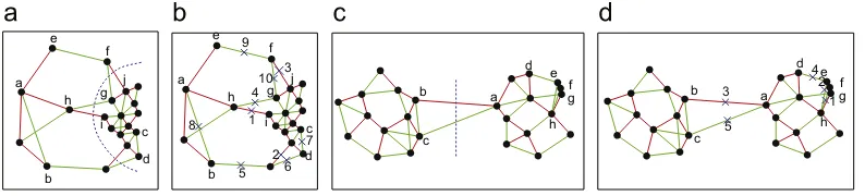
neck

a

b

c

cut1 cut2 cut3

b

c

a

c

a b

Fig. 9.Clustering a touching problem. (a) is the dataset fromFig. 1. (b) illustrates the first round of MST. (c) represents the second of MST. Comparingcut1 ofT1in (d) and cut3 ofT2in (f), two inconsistent vertices (a,c) exist, while betweencut2 in (e) andcut3 in (f), there also exist two inconsistent vertices (b,c).

Therefore, the weight ofeabin Definition 7 is redefined as

w(eab)=

×

(eab)−min(avg(E′a−{e′a}),avg(E′b−{e ′ b}))

(eab)

+(1−

)×

(eab)

(5)

where E′

a =Ea − {eab}, e′a = arg maxe∈E′

a(

(e)), E

′

b = Eb − {eab},

e′

b = arg maxe∈E′b(

(e)),

is a penalty factor and 0

ⱕ

1. E′

a− {e′a} andE′b− {e ′

b} ignore the longest neighbor edges, while

penalty factor

gives a tradeoff between the ratio and the edge length.

Fig. 8illustrates the first graph cut of applying redefined weight on the three datasets inFigs. 4–6. The correspondingRatio(Egcut)'s

are 0.500, 0.380, 0.240, respectively. According to the discussion of

in Section 4, the first two graph cuts are still valid and the third one is still invalid.

A subgraph partitioned from a separated problem may be an-other separated problem. Therefore, we must apply the graph cut method to every produced subgraph iteratively to check whether or not it can be further partitioned until no subgraphs are separated.

Algorithm 1. Clustering separated cluster problems

Input:G(X)=(V,E), the graph of the dataset to be partitioned Output:S, the set of partitioned subdatasets.

Step 1. ComputeT1andT2ofG(X), and combine the two MSTs to

construct the two-round-MST based graphGmst(X), and put it

into a table namedOpen; create another empty table named

Closed.

Step 2. If tableOpen is empty, datasets corresponding to sub-graphs inClosedtable are put intoS; returnS.

Step 3. Get a graphG′₍_X′₎₌₍_V′_,_E′_{) out of}_Open_{table, calculate the}

weights of edges inG′₍_X′_{) with Eq. (5), and build the list}

Rank(E′_).

Step 4. Remove the edges ofG′₍_X′_{) in the order of}_Rank₍_E′_{) until a}

cut is achieved.

Step 5. If the cut is valid in terms of Definition 9, put the two sub-graphs produced by the cut intoOpentable; otherwise put graphG′₍_X′_{) into}_Closed_table.

Step 6. Go to Step 2.

Algorithm 1iteratively checks subgraphs, and partitions the sep-arated ones until there exists no sepsep-arated subgraphs. At the same

(8)

neck

cut1

cut2

cut3

cut4 cut5

cut6

cut7 cut8

Fig. 10.A teapot dataset as a touching problem. (a) is a teapot dataset with a neck. In (b), the diameter defined by Zahn[18]is illustrated by the blue path.cut5 in (b) andcut7 in (c) are similar (=1), so arecut1 andcut2,cut6 andcut2,cut1 andcut8,cut3 andcut4.

time, the algorithm takes no action on non-separated subgraphs, namely touching subgraphs. In fact, the reason why Algorithm 1 can identify separated clusters is the definition of edge weight in Definition 7. The weight of an edgeeabreflects the relation between

the length ofeaband two neighbor region densities of verticesaand

b, respectively, where the neighbor region density is measured by the average length of the edges in the region. If the weight ofeabis

large, the densities of the two neighbor regions are high compared to the length

(eab), or the two densities are very different. For a

pair of touching clusters, as a neck exists and lengths of edges in the neck are small compared to the neighbor region densities, namely the weights of edges in the neck are small, Algorithm 1 cannot de-tect the touching clusters.

3.3. Algorithm for touching cluster problem

Although Algorithm 1 can identify separated clusters, it becomes disabled for touching clusters. After the algorithm is applied to a dataset, each induced sub-dataset will be either a touching cluster or a basic cluster which cannot be partitioned further.

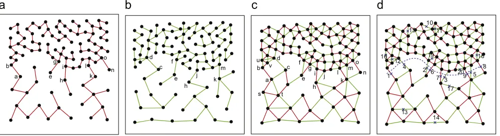
For a touching cluster, a neck exists between the two connected subclusters. The neck of touching cluster problem inFig. 1(h) is il-lustrated inFig. 9(a). Zahn[18]defined a diameter of MST as a path with the most number of edges, and detected the neck using diam-eter histogram. However, a diamdiam-eter does not always pass through a neck.Fig. 10illustrates an exception. We identify the neck by con-sideringT1andT2simultaneously. The two-round-MSTs ofFig. 1(h)

are depicted byFig. 9(b) and (c), respectively. The task in this phase is to detect and remove these edges crossing the neck, and discover touching clusters. Based on the two-round-MSTs, an important ob-servation is as follows:

Observation 1. A partition resulted from deleting an edge crossing the neck inT1is similar to a partition resulted from deleting an edge

crossing the neck inT2.

On the contrary, for the two cuts from T1 and T2,

respec-tively, if one cut does not cross the neck, the two corresponding partitions will be generally quite different from each other. Com-paring the partition onT1 inFig. 9(d) with the partition onT2 in Fig. 9(f), we notice that only two vertices (aandc) belong to dif-ferent group, and is calledinconsistent vertices. Similarly, only two

inconsistent vertices (b and c) exist between the cuts in Fig. 9(e) and (f).

For the purpose of determining whether two cuts are similar, the number ofinconsistent verticesmust be given out as a constraint, i.e. if the number ofinconsistent verticesbetween two cuts is not greater than a threshold, say

, the two cuts are similar. For the previous example inFig. 9,

=2 is reasonable. However, some unexpected pairs of cuts which do not cross the neck of a dataset may conform to the criterion and are determined to be similar. For example, thecut3 inFig. 10(b) and thecut4 inFig. 10(c) are similar if

=1, however, the two cuts are unexpected. Fortunately, the following observation can remedy this bad feature.

Observation 2. With a same threshold

, the number of pairs of similar cuts which cross the neck is generally greater than that of pairs of similar cuts which do not cross the neck.

InFig. 10(b) and (c), suppose

=1, it is easy to find another pair of similar cuts which cross the necks other thancut1 andcut2, for instance,cut5 and cut7,cut6 andcut2,cut1 andcut8, while there exists no other pair of similar cuts near cut3 andcut4. Therefore, cut3 andcut4 are discarded because the similar evidence is insuf-ficient. With the observation in mind, we can design the algorithm for touching cluster problems as follows.

Definition 10. LetPT1_{be the list of}_N₋_{1 partitions on}_T₁_{as in}

PT1₌₍_pT1 11,p

T1 12), (p

T1 21,p

T1 22), . . . , (p

T1 (N−1)1,p

T1

(N−1)2) (6)

where pair (pT1 i1,p

T1

i2) denotes the partition which results from

re-moving the i th edge in T1, pT_i11 andp T1

i2 are subsets of vertices, pT1

i1∪p T1 i2=V,|p

T1 i1|

ⱕ

|p

T1

i2|. Similarly, the list ofN−1 partitions onT2,PT2,

is defined as

PT2₌₍_pT2 11,p

T2 12), (p

T2 21,p

T2 22), . . . , (p

T2 (N−1)1,p

T2

(N−1)2) (7)

Obviously, some partitions both onT1andT2can be very skewed.

However, a valid partition is expected to generate two subsets with relatively balanced element numbers in some typical graph partition methods, such as ratio cut[32]. Therefore, the partition listsPT1_and PT2_{can be refined by ignoring skewed partitions so as to reduce the}

number of comparisons.

Definition 11. LetRPT1 _and_RPT2_{be the refined lists, all of the}

ele-ments ofRPT1_{come from}_PT1_{, and all of the elements of}_RPT2_come

(9)

5 10 15 20 25 30

Fig. 11.Clustering results on DS1. (a) is the original dataset; (b) is the clustering result ofk-means; (c) is the clustering result of DBScan (MinPts=3, Eps=1.6); (d) is the clustering result of single-linkage; (e) is the clustering result of spectral clustering; (f) is the clustering result of 2-MSTClus.

fromPT2_{, as in}

In the next step, partitions inRPT1_{will be compared with those in} RPT2_{. As the number of}_{inconsistent vertices}_{between two cuts must}

be less than or equal to the threshold

, if||rpT1 i1| − |rp

T2

j1||

>

, the

comparison between two partitions (rpT1 i1,rp

For the purpose of saving the computational cost, we can further combine the two listsRPT1_and_RPT2_{, and order them ascendingly by}

the element numbers of the left parts of the pairs. Only pairs which come from different MSTs and of which element number of left parts have differences not more than

will be compared.

Definition 12. LetSPbe a set which consists of all the elements of RPT1 _and_RPT2_: source ofspis defined as

source(sp)=

the ordered list as in

CP(SP)= part_ min(SP)◦CP(SP− {part_ min(SP)}) (12) wherepart_ min(SP)=arg minsp∈SP|left(sp)|, and◦is a concatenate

operator.

Definition 15. Two partitions (cp_i1,cpi2) and (cpj1,cpj2) are said to

be similar, wherei

ⱕ

j, if the followings hold:

(a) source((cpi1,cpi2))

source((cpj1,cpj2));

(b) |cp_i1−cpj1| + |cpj1−cpi1|

ⱕ

or|cpi1−cpj2| + |cpj2−cpi1|

ⱕ

.

The first condition indicates that the two partitions come from different MSTs, while the second condition reveals that the number of inconsistent vertices between the two partitions is sufficient small.

(10)

5 10 15 10

12 14 16 18 20 22 24 26

5 10 15

10 12 14 16 18 20 22 24 26

5 10 15

10 12 14 16 18 20 22 24 26

5 10 15

10 12 14 16 18 20 22 24 26

5 10 15

10 12 14 16 18 20 22 24 26

5 10 15

10 12 14 16 18 20 22 24 26

Algorithm 2. Clustering touching problems

Input:T1andT2, the two rounds of MST of a sub-dataset generated

byAlgorithm 1.

Output:S, the set of expected partitions.

Step 1. Construct the ordered listCP(SP) withT1andT2; create two

empty setS′_and_S_.

Step 2. For each (cp_i1,cpi2)∈CP(SP), it is compared with (cpj1,cpj2)∈ CP(SP) andj

>

i. According to Definition 15, if there exists a partition (cpj1,cpj2) which is similar to (cpi1,cpi2), (cpi1,cpi2)

is put intoS′_.

Step 3. For eachs∈S′_{, if there exists a}_t_∈_S′_,_t

_s_{, and}_t_{is similar to}

s,sis put intoS.

Step 4. Combine similar partitions inS.

In Algorithm 2, Step 3 is to remove the unexpected partitions in terms of Observation 2. For simplicity, only those partitions without similar others are removed. In Step 3, when determining the simi-larity betweentands, we ignore whether they come from different MSTs or not, since at this stage only the number of inconsistent ver-tices are concerned. Step 4 combines the similar partitions. This can be achieved by assigninginconsistent verticesto two groups in terms of the evidence (support rate) accumulated from the similar parti-tions. Algorithm 2 can identify touching clusters except overlapping ones.

3.4. The combination of the two algorithms

As mentioned above, cluster problems are categorized into sep-arated problems and touching problems in this paper, and the two cluster problems roughly cover all the cluster problems since they are mutual complementary. As Algorithm 1 automatically identifies separated clusters and has no effect on touching clusters, Algorithms 1 and 2 can be easily combined to deal with any cluster problem. When every subset partitioned by Algorithm 1 is fed to Algorithm 2, we will obtain the final clustering results. Therefore, the two al-gorithms can be easily combined to form the method 2-MSTClus.

Many traditional clustering algorithms are vulnerable to the dif-ferent cluster sizes, shapes and densities. However, since the sepa-rated clusters and touching clusters can roughly cover all kinds of clusters (except overlapping clusters) in terms of definition of sep-arated cluster and touching cluster regardless of cluster size, shape and density, the combination of Algorithms 1 and 2 is robust to di-versifications of sizes, shapes and densities of clusters.

3.5. Computational complexity analysis

The computational complexity of Algorithm 1 is analyzed as fol-lows. For a graphG(X)=(V,E), if Fibonacci heaps are used to im-plement the min-priority queue, the running time of Prim's MST

(11)

2 4 6 8 10 12 14 16 10

12 14 16 18 20 22 24 26

2 4 6 8 10 12 14 16

10 12 14 16 18 20 22 24 26

2 4 6 8 10 12 14 16

10 12 14 16 18 20 22 24 26

2 4 6 8 10 12 14 16

10 12 14 16 18 20 22 24 26

2 4 6 8 10 12 14 16

10 12 14 16 18 20 22 24 26

2 4 6 8 10 12 14 16

10 12 14 16 18 20 22 24 26

Fig. 13.Clustering results on DS3. (a) is the original dataset; (b) is the clustering result ofk-means; (c) is the clustering result of DBScan (MinPts=5, Eps=1.5); (d) is the clustering result of single-linkage; (e) is the clustering result of spectral clustering; (f) is clustering result of 2-MSTClus.

algorithm isO(|E| + |V|log|V|)[35]. As the MST in a graph-based clustering method is generally constructed from a complete graph,

|E|is equal to|V|2and the computational complexity of Prim's algo-rithm isO(|V|2). In Step 1, accordingly,T1 andT2 are generated in O(N2_{), while Step 3 sorts the list}_Rank₍_E′_{) in}_O₍_N_log_N_{). Step 4}

re-peatedly removes an edge ofG′₍_X′_{) and checks if a cut is achieved}

inO(|X′_|_log_|_X′_|_{), where}_|_X′_|

_ⱕ

_N_{. The iteration time from Step 2 to}

Step 6 is the number of separated clusters in dataset, which is gen-erally far less thanN. Therefore, the time complexity of Algorithm 1 isO(N2_).

In Step 1 of Algorithm 2, the constructingSPtakesO(N2), and sortingCP(SP) takesO(NlogN). As a result, the Step 1 can be done inO(N2_{). The iteration in Step 2 of Algorithm 2 can be finished in} O(NlogN). Both Steps 3 and 4 in Algorithm 2 are executed inO(N). The computational complexity of Algorithm 2 isO(N2_).

Obviously, since the method 2-MSTClus is composed of Algorithms 1 and 2, its overall time complexity isO(N2_).

4. Experimental results

4.1. Parameter setting

In the two proposed algorithms, although four parameters exist, they are all set to fixed values in all our experiments. The parameter

determines whether a graph cut is valid or not when the framework

deals with separated cluster problems. For the first graph cut on a separated problem, the numbers of edges removed fromT1and T2, respectively, are almost equal. The ideal situation is that two

clusters are far away from each other, and when the first graph cut is achieved the number of the edges removed from T1 is equal to

that of the edges fromT2, i.e.

=0.5. For non-separated problems,

on the contrary, the edges removed fromT2are in the majority, and

that leads to significantly skewed ratio. However, a change of local density may disturb the ratio. Accordingly the parameter

is relaxed to some degree. In all of our experiments, the parameter is set to 0.330. Specially, suppose that three edge removals result in a cut, although theRatio(Egcut) is 0.333 and only slightly greater than the

parameter, the absolute difference is very small (only 1).

When the weight of an edge is computed, the parameter

is employed to balance the relative weight (the ratio of lengths) and the absolute weight (the length of the edge). As the relative weight is crucial,

is generally set to 0.9.

In touching problem algorithm, the parameter

is the margin of the number ofinconsistent vertices. If it is too small, some neck-crossed partitions may be identified as invalid, while if it is too large, some non-neck-crossed partitions may be regarded as valid. As overlapped clusters are beyond the scope of this paper, and only slightly touching clusters are considered,

is set to a relatively small value, for instance, 2 in all our experiments. In addition, some ex-treme skewed partitions can be ignored by the parameter

to save

(12)

5 10 15 20 25 30 35 0

5 10 15 20 25 30

5 10 15 20 25 30 35

0 5 10 15 20 25 30

5 10 15 20 25 30 35

0 5 10 15 20 25 30

5 10 15 20 25 30 35

0 5 10 15 20 25 30

5 10 15 20 25 30 35

0 5 10 15 20 25 30

5 10 15 20 25 30 35

0 5 10 15 20 25 30

Fig. 14.Clustering results on DS4. (a) is the original dataset; (b) is the clustering result ofk-means; (c) is the clustering result of DBScan (MinPts=6, Eps=1.5); (d) is the clustering result of single-linkage; (e) is the clustering result of spectral clustering; (f) is clustering result of 2-MSTClus.

the computational cost in touching problem algorithm. For example, cuts on some short branches (called hairs by[18]) are meaningless. Although the short branches can be identified adaptively, for sim-plicity we set

∈[0.01, 0.05] in the following experiments. If the number of vertices contained in a short branch is less than

vertices, cuts on the short branch will be ignored.

4.2. Experiments on synthetic and real datasets

The proposed method 2-MSTClus is tested on five 2-D synthetic datasets, DS1–DS5, and two UCI datasets, Iris and Wine, and com-pared with four typical clustering algorithms, namely k-means, DBScan, single-linkage and spectral clustering, in which normalized cut is used. For DBScan, in the all experiments, the parameters are selected with the best clustering result.

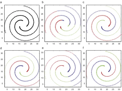
The dataset DS1 is taken from[34]and illustrated inFig. 11(a). It contains three spiral clusters, which are separated from each other in distance, therefore it is a distance-separated cluster problem. How-ever, in terms of Handl's taxonomy[12], DS1 falls into the group of connectedness.Fig. 11(b)–(f) depict the clustering results of the four methods and 2-MSTClus. As DBScan and single-linkage prefer the datasets with connectedness, they can discover the three actual clusters, butk-means and spectral clustering cannot. 2-MSTClus can easily deal with DS1 as a separated problem and detect the three clusters.

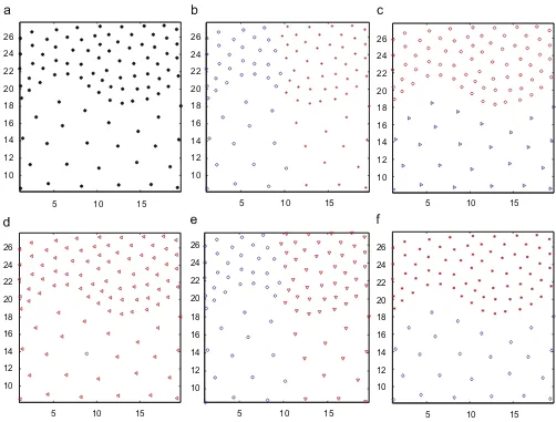
Fig. 12illustrates the clustering results of DS2, which is from[18]. It is a typical density-separated cluster problem. Since DBScan is a based and identifies clusters with the concept of density-reachable, it partitions DS2 well. However,k-means, single-linkage and spectral clustering are ineffective on DS2. While 2-MSTClus still produces ideal result by its separated algorithm.

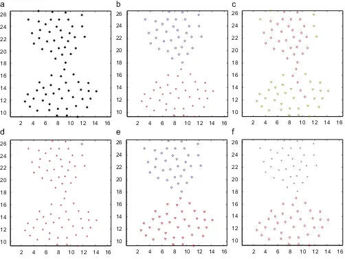
The dataset DS3 is also taken from [18] and illustrated in

Fig. 13. It is composed of two clusters, which are compact and slightly touched.k-means, which favors this kind of dataset, and spectral clustering have good performance on D3, whereas single-linkage and DBScan perform badly. Instead of the separated algorithm of 2-MSTClus, the touching algorithm of 2-MSTCLus can detect the two clusters.

InFig. 14(a), the dataset DS4 is taken from[11]. Compared with the former three datasets DS1–DS3, this dataset is more complex. It consists of seven clusters, and is a composite cluster problem. All of the four algorithms,k-means, DBScan, single-linkage, spectral clustering fail on this dataset. However, 2-MSTClus identifies the seven clusters accurately.

In DS4, three clusters are distance-separated from others, while two pairs are internal touched. When the dataset is fed to 2-MSTClus, Algorithm 1 is first applied to it.Fig. 15(a) represents the first cut when top two weight edges are removed. As theRatio(Egcut) is 0.333,

and greater than the threshold

, the cut is valid. Next cut analysis is on the remaining six clusters. InFig. 15(b), the removals of the top

(13)

1 2 3

cut4 _cut10

cut3 cut9

cut2

cut1 _cut8

cut1

cut2 cut3

cut4 cut5

cut6 1

2

1 2

cut5 cut6

cut7

cut11

cut7

cut8 1 2

Fig. 15.Clustering process of 2-MSTClus on DS4. (a)–(d) illustrate the four graph cuts by the separated algorithm. In (e) and (f), Algorithm 2 is applied,cut1 andcut8,cut2 andcut9,cut3 andcut9,cut4 andcut9,cut5 andcut10,cut6 andcut11,cut7 andcut11,are similar (=2). In (g) and (h),cut1 andcut2,cut3 andcut6,cut5 andcut2,cut7 andcut2,cut4 andcut4, etc. are similar (=2).

two edges result in a valid cut, which partitions the six clusters into two groups. Similarly, the separated sub-dataset inFig. 15(c) and (d) is further partitioned. Afterwards, Algorithm 1 could not partition the clusters any more. Then all the clusters are checked by Algorithm 2. Two touching clusters problems are figured out inFig. 15(e)–(h), even though inFig. 15(g) and (h) the two clusters have significant difference in their sizes.

The dataset DS5 is composed of three datasets from[18]. The left top dataset inFig. 16(a) is a touching problem; the left bottom one is a distance-separated problem; while the right one is a density-separated problem. For this composite dataset, 2-MSTClus can iden-tify the six clusters, but the four clustering methodsk-means, single-linkage, DBScan and spectral clustering cannot.

InFig. 17(a), (b) and (d), the distance-separated problems are identified with the removals of top two edges, respectively. With diverse densities, the two clusters inFig. 17(c) are partitioned by Algorithm 1, and the correspondingRatio(Egcut) is 0.417, hence the

graph cut is valid. As for the touching problem in the top left of

Fig. 16(a), Algorithm 1 is ineffective. The similar cuts inFig. 17(e) and (f) are detected by Algorithm 2.

Two real datasets from UCI are employed to test the proposed method. The first one is IRIS, which is a well-known benchmark for machine learning research. The dataset consists of three clusters with 50 samples each, and the one is well separated from the other two clusters, while the two clusters are slightly touched to each other. Similar to DS4 and DS5, it is also a composite clustering problem. When the dataset is fed to the 2-MSTClus, Algorithm 1 in the first round cuts off 50 samples, which constitute the separated cluster.

Then the algorithm produces no clusters further. When Algorithm 2 is applied to the two subsets, only the cluster that is composed of 100 samples has some similar cuts between itsT1andT2, therefore,

this cluster is further partitioned.

The performance comparison on IRIS is presented inTable 1. Four frequently-used external clustering validity indices are employed to evaluate the clustering results: Rand, Adjusted rand, Jaccard and FM. FromTable 1, it is evident that 2-MSTClus performs best, since all of indices of 2-MSTClus are ranked first.

The second real dataset is WINE. It is composed of 178 samples, which fall into three clusters. From Table 2, 2-MSTClus performs only better than single-linkage. Compared with the former datasets, the performance of 2-MSTClus on WINE is slightly weakened. This is because some outliers exist in the dataset. In Algorithm 1, the graph cut criterion is a heuristic, however, the existence of outlier may affect the heuristic.

5. Discussion

Traditional MST-based clustering methods [18,19,24,33] make use of an MST to partition a dataset. A general way of partitioning is to remove the edges with relative large lengths, and one removal leads to a bipartition. Within an MST, although some crucial infor-mation of a dataset are collected, some are missed. T1 andT2 are

combined to form a graph for the purpose of accumulating more evidence to partition datasets. In a two-round-MST based graph, a graph cut requires at least two edge removals. Only the evidence fromT1andT2being consistent, is the graph cut valid. For analyzing

(14)

10 15 20 25 30 35 40 5

10 15 20 25

10 15 20 25 30 35 40

5 10 15 20 25

10 15 20 25 30 35 40

5 10 15 20 25

10 15 20 25 30 35 40

5 10 15 20 25

10 15 20 25 30 35 40

5 10 15 20 25

10 15 20 25 30 35 40

5 10 15 20 25

2

1

7 21

3 23

13 18 1

14 11

16 17 4 2

6 12 9 10

8 19 24 5

22

15 20

1 2

2 1

cut1

cut5 cut4

cut7

cut2 cut3

cut6

Fig. 17.Clustering process of 2-MSTClus on DS5. In (a), (b) and (d), the separated clustering method is applied. Only two edges are removed for each dataset and three valid graph cuts are achieved. (c) illustrates the partitioning process of the density-separated cluster problem. Totally 24 edges are removed for the graph cut, from which 14 edges come fromT2and 10 fromT1. In (e) and (f),cut1 andcut5,cut1 andcut6,cut2 andcut7,cut3 andcut7,cut4 andcut7 are similar (=2).

the touching problems in 2-MSTClus, the concept ofinconsistent ver-ticesdelivers the same idea.

The proposed method 2-MSTClus deals with a dataset in terms of which cluster problem it belongs to, separated problem or touching problem. The diversifications of sizes, shapes as well as densities of clusters have no effect on the clustering process.

A drawback of 2-MSTClus is that it is not robust to outliers. Al-though some outlier detection methods can be used to preprocess a dataset and remedy this drawback, we will discover more robust mechanism to outliers based on two-round-MST based graph in the future. In addition, the proposed method cannot detect the overlap-ping clusters. If a dataset composed of two overlapoverlap-ping clusters is

(15)

Performance comparison on IRIS data.

Method Rand Adjusted rand Jaccard FM

k-Means 0.8797 0.7302 0.6959 0.8208

DBScan 0.8834 0.7388 0.7044 0.8268

Single-linkage 0.7766 0.5638 0.5891 0.7635

Spectral clustering 0.7998 0.5468 0.5334 0.6957

2-MSTClus 0.9341 0.8512 0.8188 0.9004

Table 2

Performance comparison on WINE data.

Method Rand Adjusted rand Jaccard FM

k-Means 0.7183 0.3711 0.4120 0.7302

DBScan 0.7610 0.5291 0.5902 0.7512

Single-linkage 0.3628 0.0054 0.3325 0.5650

Spectral clustering 0.7644 0.4713 0.4798 0.6485

2-MSTClus 0.7173 0.3676 0.4094 0.5809

dealt with 2-MSTClus, the two clusters will be recognized as one cluster.

If more MSTs are combined, for instance,T1,T2,T3, . . . ,Tk,k

ⱕ

N/2,

does the performance of the proposed method become better? In other words, how is a suitablekselected for a dataset? This is an interesting problem for the future work.

6. Conclusions

In this paper, a two-round-MST based graph is utilized to repre-sent a dataset, and a clustering method 2-MSTClus is proposed. The method makes use of the good properties of the two-round-MST based graph, automatically differentiates separated problems from touching problems, and deals with the two kinds of cluster problem. It does not request user-defined cluster number, and is robust to dif-ferent cluster shapes, densities and sizes. Our future work will focus on improving the robustness of 2-MSTClus to outliers and selecting a reasonablekfor constructingk-MST.

Acknowledgments

We would like to thank the anonymous reviewers whose thoughtful comments and suggestions improved the quality of this paper. The paper is supported by the National Natural Science Foundation of China, Grant No. 60775036, No. 60475019, and the Research Fund for the Doctoral Program of Higher Education: No. 20060247039.

References

[1] W. Cai, S. Chen, D. Zhang, Fast and robust fuzzy c-means clustering algorithms incorporating local information for image segmentation, Pattern Recognition 40 (2007) 825–838.

[2] Z. Wu, R. Leahy, An optimal graph theoretic approach to data clustering: theory and its application to image segmentation, IEEE Transactions on Pattern Analysis and Machine Intelligence 15 (1993) 1101–1113.

[3] J. Han, M. Kamber, Data Mining: Concepts and Techniques, Morgan-Kaufman, San Francisco, 2006.

from gene expression data, Bioinformatics 23 (2007) 2888–2896.

[5] S. Bandyopadhyay, A. Mukhopadhyay, U. Maulik, An improved algorithm for clustering gene expression data, Bioinformatics 23 (2007) 2859–2865. [6] A.K. Jain, M.C. Law, Data clustering: a user's dilemma, Pattern Recognition and

Machine Intelligence, Lecture Notes in Computer Science, 3776, Springer, Berlin, Heidelberg, 2005, pp. 1–10.

[7] R. Xu, D. Wunsch II, Survey of clustering algorithms, IEEE Transactions on Neural Networks 16 (2005) 645–678.

[8] J. Kleinberg, An Impossibility Theorem for Clustering, MIT Press, Cambridge, MA, USA, 2002.

[9] H.G. Ayad, M.S. Kamel, Cumulative voting consensus method for partitions with variable number of clusters, IEEE Transactions on Pattern Analysis and Machine Intelligence 30 (2008) 160–173.

[10] A. Topchy, A.K. Jain, W. Punch, Clustering ensembles: models of consensus and weak partitions, IEEE Transactions on Pattern Analysis and Machine Intelligence 27 (2005) 1866–1881.

[11] A. Gionis, H. Annila, P. Tsaparas, Clustering aggregation, ACM Transactions on Knowledge Discovery from Data 1 (2007) 1–30.

[12] J. Handl, J. Knowles, An evolutionary approach to multiobjective clustering, IEEE Transactions on Evolutionary Computation 11 (2007) 56–76.

[13] A.L. Fred, A.K. Jain, Combining multiple clusterings using evidence accumulation, IEEE Transactions on Pattern Analysis and Machine Intelligence 27 (2005) 835–850.

[14] N. Bansal, A. Blum, S. Chawla, Correlation clustering, Machine Learning 56 (2004) 89–113.

[15] G.V. Nosovskiy, D. Liu, O. Sourina, Automatic clustering and boundary detection algorithm based on adaptive influence function, Pattern Recognition 41 (2008) 2757–2776.

[16] G. Karypis, E.H. Han, V. Kumar, CHAMELEON: a hierarchical clustering algorithm using dynamic modeling, IEEE Transactions on Computers 32 (1999) 68–75. [17] P. Fr¨anti, O. Virmajoki, V. Hautamaki, Fast agglomerative clustering using a¨

k-nearest neighbor graph, IEEE Transactions on Pattern Analysis and Machine Intelligence 28 (2006) 1875–1881.

[18] C.T. Zahn, Graph-theoretical methods for detecting and describing gestalt clusters, IEEE Transactions on Computers C-20 (1971) 68–86.

[19] Y. Xu, V. Olman, D. Xu, Clustering gene expression data using a graph-theoretic approach: an application of minimum spanning tree, Bioinformatics 18 (2002) 536–545.

[20] J.M. González-Barrios, A.J. Quiroz, A clustering procedure based on the comparison between theknearest neighbors graph and the minimal spanning tree, Statistics & Probability Letters 62 (2003) 23–34.

[21] N. P¨aivinen, Clustering with a minimum spanning tree of scale-free-like structure, Pattern Recognition Letters 26 (2005) 921–930.

[22] J. Shi, J. Malik, Normalized cuts and image segmentation, IEEE Transactions on Pattern Analysis and Machine Intelligence 22 (2000) 888–905.

[23] C.H. Lee, et al., Clustering high dimensional data: a graph-based relaxed optimization approach, Information Sciences 178 (2008) 4501–4511. [24] S. Bandyopadhyay, An automatic shape independent clustering technique,

Pattern Recognition 37 (2004) 33–45.

[25] G.T. Toussaint, The relative neighborhood graph of a finite planar set, Pattern Recognition 12 (1980) 261–268.

[26] J. Handl, J. Knowles, D.B. Kell, Computational cluster validation in post-genomic data analysis, Bioinformatics 21 (2005) 3201–3212.

[27] M. Steinbach, L. Ertoz, V. Kumar, The Challenges of Clustering High Dimensional¨ Data, New Directions in Statistical Physics: Bioinformatics and Pattern Recognition, L.T. Wille (Ed.), Springer, Berlin, 2002, pp. 273–307.

[28] A.K. Jain, R.C. Dubes, Algorithms for Clustering Data, Prentice-Hall, Englewood Cliffs, NJ, 1988.

[29] B. Fischer, J.M. Buhmann, Path-based clustering for grouping of smooth curves and texture segmentation, IEEE Transactions on Pattern Analysis and Machine Intelligence 25 (2003) 513–518.

[30] L. Yang, K-edge connected neighborhood graph for geodesic distance estimation and nonlinear data projection, in: Proceedings of the 17th International Conference on Pattern Recognition (ICPR'04), 2004.

[31] U. Brandes, M. Gaertler, D. Wagner, Engineering graph clustering: models and experimental evaluation, ACM Journal of Experimental Algorithmics 12 (2007). [32] L. Hagen, A.B. Kahng, New spectral methods for ratio cut partitioning and clustering, IEEE Transactions on Computer-Aided Design 11 (1992) 1074–1085. [33] Y. Li, A clustering algorithm based on maximal -distant subtrees, Pattern

Recognition 40 (2007) 1425–1431.

[34] H. Chang, D.Y. Yeung, Robust path-based spectral clustering, Pattern Recognition 41 (2008) 191–203.

[35] T.H. Corman, C.E. Leiserson, R.L. Rivest, C. Stein, Introduction to Algorithms, second ed., MIT press, Cambridge, MA, 2001.

About the Author—CAIMING ZHONG is currently pursuing his Ph.D. in Computer Sciences at Tongji University, Shanghai, China. His research interests include cluster analysis, manifold learning and image segmentation.

About the Author—DUOQIAN MIAO is a professor of Department of Computer Science and Technology at Tongji University, Shanghai, China. He has published more than 40 papers in international proceedings and journals. His research interests include soft computing, rough sets, pattern recognition, data mining, machine learning and granular computing.

About the Author—RUIZHI WANG is a Ph.D. candidate of Computer Sciences at Tongji University of China. Her research interests include data mining, statistical pattern recognition, and bioinformatics. She is currently working on biclustering algorithms and their applications to various tasks in gene expression data analysis.