www.elsevier.nlrlocaterjappgeo
Ground penetrating radar inversion in 1-D: an approach for the
estimation of electrical conductivity, dielectric permittivity and
magnetic permeability
1O. Lazaro-Mancilla
´
), E. Gomez-Trevino
´
˜
( )
Departamento de Geofısica Aplicada, Centro de In´ Õestigacion Cientıfica y de Educacion Superior de Ensenada CICESE ,´ ´ ´ Km 107 Carretera Tijuana-Ensenada, Ensenada, B.C. 22800, Mexico
Received 15 September 1998; received in revised form 22 February 1999; accepted 15 March 1999
Abstract
This paper presents a method for inverting ground penetrating radargrams in terms of one-dimensional profiles. We resort to a special type of linearization of the damped E-field wave equation to solve the inverse problem. The numerical algorithm for the inversion is iterative and requires the solution of several forward problems, which we evaluate using the matrix propagation approach. Analytical expressions for the derivatives with respect to physical properties are obtained using the self-adjoint Green’s function method. We consider three physical properties of materials; namely dielectrical permittivity, magnetic permeability and electrical conductivity. The inverse problem is solved minimizing the quadratic norm of the residuals using quadratic programming optimization. In the iterative process to speed up convergence we use the Levenberg–Mardquardt method. The special type of linearization is based on an integral equation that involves derivatives of the electric field with respect to magnetic permeability, electrical conductivity and dielectric permittivity; this equation is the result of analyzing the implication of the scaling properties of the electromagnetic field. The ground is modeled using thin horizontal layers to approximate general variations of the physical properties. We show that standard synthetic radargrams due to dielectric permittivity contrasts can be matched using electrical conductivity or magnetic permeability variations. The results indicate that it is impossible to differentiate one property from the other using GPR data.q2000
Elsevier Science B.V. All rights reserved.
Keywords: Ground penetrating radar; Frechet derivatives; Inverse problem; Parameter estimation; Quadratic programming´
)
Corresponding author. Department of Applied Geo-physics, CICESE, P.O. Box 434843, San Diego, CA 92143-4843, USA. Fax: q1-526-174-4880; e-mail: [email protected]
1
Paper presented at Seventh International Conference on Ground Penetrating Radar, May 27–30, 1998. Univer-sity of Kansas, Lawrence, KS, USA.
1. Introduction
Ž .
Given a ground penetrating radar GPR sig-nal or radargram, it is of interest to determine all the possible information about the subsurface features that gave origin to the signal. In terms of a physical model of the ground, we need to estimate the parameters of the model. This rep-resents an inverse problem. For the case of
0926-9851r00r$ - see front matterq2000 Elsevier Science B.V. All rights reserved. Ž .
GPR, the problem is nonlinear and besides it requires to invert for the three physical proper-ties of materials; namely magnetic permeability, electric conductivity and dielectric permittivity, all as functions of depth. The purpose of this paper is to demonstrate that an integral equation formulation of the one-dimensional GPR in-verse problem can be used to recover any of the three physical properties.
The scaling properties of Maxwell’s equa-tions allow the existence, for the case of quasi-static fields, of simple integral equations for
Ž .
electrical conductivity Gomez-Trevino, 1987 .
´
˜
These equations were developed in an attempt to reduce the generality of linearization to the exclusive scope of electromagnetic problems. The reduction is achieved when the principle ofŽ
similitude for quasi-static fields neglecting dis-.
placement currents is imposed on linearized forms of the field equations. The combination leads to exact integral relations that represent a unifying framework for the general electromag-netic inverse problem. The constructed formula-tion is exact and preserves the nonlinear depen-dence of the model and the data. Iterating the integral equations, it is possible to recover a conductivity distribution from a given set of data. This was demonstrated by Esparza and
Ž .
Gomez-Trevino 1996; 1997
´
˜
for magnetotel-luric and direct current resistivitymeasure-Ž .
ments. In the work of Gomez-Trevino 1999 ,
´
˜
the equations for quasi-static fields are general-ized by the inclusion of displacement currents. Our inverse procedure is based on the general equations that involve the three electromagnetic properties of materials.We consider 1-D profiles and assume a plane wave approximation. The algorithm is iterative and for the multiple evaluation of the forward problem we use the matrix propagation ap-proach as described by Lazaro-Mancilla and
´
Ž .
Gomez-Trevino
´
˜
1996 . We present analytic derivatives of the electric field with respect to the three physical properties. The self-adjoint Green’s function method as described byŽ .
McGillivray and Oldenburg 1990 is applied in
the derivations. The inverse problem is solved using quadratic programming. In this we follow
Ž .
Gill et al. 1986 . To ensure convergence we
apply the Levenberg–Mardquardt method
ŽLevenberg, 1944; Mardquardt, 1963 ..
We present some examples of parameter esti-mation and show how a synthetic radargram due to dielectric permittivity variations can be inter-preted as if it were produced by magnetic per-meability contrasts which, although not impos-sible to find in nature, they may in practice be very unlikely to occur. Magnetic permeability variations are commonly neglected because in most GPR applications the magnetic character-istics of geological materials are seldom differ-ent from those of free space. However, signifi-cant permeability variations can be associated to horizontal layers with high concentrations of magnetic minerals in a paleo-beach environ-ment, enriched in hematite or limonite which are produced by chemical alterations of mag-netite or titanomagmag-netite, heavy minerals whose relative permeabilities may vary from 1.0064 to
Ž .
6.5 Rzhevsky and Novik, 1971 . The radar-grams due to permittivity variations may also be explained by electrical conductivity contrasts. In this case, the ambiguity is more likely to occur in practice given the wide range of variation of this property.
2. Theory
2.1. Forward problem
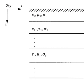
Consider a plane wave at normal incidence upon an n-layer earth model as illustrated in Fig. 1. The three electromagnetic properties vary from layer to layer; each layer is linear, homo-geneous and isotropic. A dependence of the form eivt is assumed for the fields, where t is time and v angular frequency. It is further assumed that the physical properties do not depend on frequency. The governing differential
Ž .
Fig. 1. Layered earth model whose three electromagnetic properties vary from layer to layer. The plane wave propa-gates downward in the positive z-direction.
Ž .
H z fields propagating in the z-direction are,y
for the ith layer:
d2
is the propagation constant of the layer. The quantities mi, si and ´i represent magnetic permeability, electrical conductivity and dielec-tric permittivity, respectively. The solution is obtained in the standard form of a boundary value problem where we consider 2 n boundary conditions and 2 n unknowns. The electric field in the ith layer is expressed in terms of an outgoing and a reflected wave, i.e.:
E sA eygizqB egiz,
Ž .
4xi i i
where A and B are coefficients that need to bei i
determined. Applying continuity of the fields at each boundary and employing standard propaga-tion matrices, we can find the fields in one layer in terms of the fields in the next layer. Setting
the amplitude of the incident wave A0s1, the electric field at the surface is given simply as:
E 0x
Ž .
s1qB .0Ž .
5The radargram is computed as in Lazaro-
´
Ž .
Mancilla and Gomez-Trevino 1996 by apply-
´
˜
ing the inverse Fourier transform to the product of the electric field and the Ricker’s pulsespec-Ž . trum S f , i.e.:
y1
EsFFT Ex
Ž . Ž .
f S f .Ž .
6A variety of examples are presented by
Ž .
Lazaro-Mancilla and Gomez-Trevino 1996 that
´
´
˜
illustrate the signatures produced by variations in m, s and ´. By trial and error methods it was possible to match radargrams due to varia-tions in one property with those produced by the other two. In the present work, we reconsider this issue from the point of view of an auto-matic fitting process.2.2. InÕerse problem
Ž .
In Gomez-Trevino
´
˜
1999 , the differential equations for the electric field E and magnetic field B are transformed to integral equations forŽ .
magnetic permeability m , electrical
conductiv-Ž . Ž .
ity s and dielectric permittivity ´ . For the electric field, the equation is:
Es G m rX d3rX Frechet derivatives of E with respect to
´
m, sand ´, respectively. E represents the data and the unknown functions are m, s and ´. The
Ž .
integral Eq. 7 is nonlinear because the func-tional derivatives depend on the physical
prop-Ž .
inte-gration of the functional derivatives of E with
We base the solution of the inverse problem on Ž .
Eq. 11 .
2.3. Analytic Frechet deri
´
ÕatiÕesA fundamental step in the solution of most nonlinear inverse problems is to establish a relationship between changes in a proposed model and corresponding changes in the data. Once this relationship is established, it becomes possible to refine an initial model to obtain an improved fit to the observations. In traditional linearized analysis, the Frechet derivative is the
´
connecting link between changes in the modelŽ .
and changes in the data. In Eq. 7 , the same derivative links directly the data to the model.
The usual approach for developing expres-sions for the Frechet derivatives is to perturb the
´
governing differential equation and thereby for-mulate a new problem that relates the change in the response to a change in the model. We derive the analytic derivatives using the self-ad-joint Green’s function method. The wave equa-tion for the case of arbitrary variaequa-tions in thephysical properties can be written from
Maxwell’s equations as:
Strictly speaking, Eq. 12 should include a
source term. However, for the purpose of the perturbation analysis that follows its inclusion is unnecessary because we consider perturbations of only the physical properties and the fields.
Ž .
Perturbing Eq. 12 , keeping only first order terms in the resulting perturbations and using
Ž .
Eq. 12 again there results:
hX hX
In the self-adjoint form:
hX
The solution of Eq. 14 can be obtained
through the use of the Green’s function for the
Ž .
layered model. Let G z, z0 be this function and
Ž .
d z, z0 the corresponding Dirac delta function.
Ž . Ž .
Integrating Eq. 15 between z0 and z0 in the usual manner, one obtains:
h z q G
We use this equation to obtain a quantitative
Ž . Ž .
relationship between G z, z0s0 and E z . For
Ž . Ž .
the moment consider that G z, z0 sG z , z .0
That is, G can be interpreted either as the field at z due to a source at z , or as the field at z0 0 due to a source at z. For convenience we choose to consider G as the field at z due to a source at z0 because this field is simply the physical field within the layered model. This
Ž . Ž .
comes from the fact that Eqs. 12 and 15 are one and the same equation, except for the loca-tion of the source. However, since we are con-sidering the case of a plane wave source, it is irrelevant whether the source is placed right on
Ž . Ž .
account for physical dimensions and differences in source strength. That is:
E z
Ž .
G z
Ž .
s ,Ž .
17C
where C is independent of depth and we have
Ž . Ž .
written G z, z0s0 sG z .
Ž . Ž .
Substituting Eq. 17 into Eq. 16 we must have:
X< X<
hE qyhE ysC.
Ž .
18The discontinuity is produced by the source
Ž X
.
at z0s0. The fact that yhEriv is simply the magnetic field of the source provides the clue for what the value of C must be. The magnetic fields produced by a plane source have the same intensity on both sides of the plane but are of different signs. Furthermore, the intensity of the magnetic field is equal to one-half the strength of the source. Using Eq. Ž .4 we can compute the magnetic field just on top of the model. The result can be written as
Ž y. XŽ y. Ž y. Ž .
h 0 E 0 sh 0 g0 B0y1 , where we
have kept A0s1 as for the computation of the electric field. The above-arguments then lead to:
Cs yh 0y EX
0y . 19
Ž
.
Ž
.
Ž .
We must then have that:
m0E z
Ž .
G z
Ž .
s .Ž .
20g0
Ž
B0y1.
We get the Frechet derivative for the 1-D GPR
´
problem through:The last two integrals are more direct to obtain than the first. To obtain the first integral
Ž it is necessary to use the wave equation Eq. Ž12.. in the intermediate steps.
Ž .
Substituting Eqs. 23 – 25 into Eqs. 8 – Ž10 , respectively, one obtains expressions for. the partial derivatives in terms of the electric field within a given layer. Considering the ex-plicit expressions for the electric field given by
Ž .
For the nth layer we have:
EE 0
Ž .
m0 1 gnA2n y2g zn n
s y 2 e .
Ž .
27Emn g0
Ž
B0y1 2.
mnFor electrical conductivity the derivatives are:
For the nth layer: For permittivity the results are:
EE 0
Ž .
m0 2and the expression for the nth layer:
EE 0
Ž .
m0 2 A2n y2g z The values of the derivatives in the time domain are obtained by applying the Fourier transform as already explained in relation to Eq. Ž .6 . We use a layered model that can be made up of many thin layers to simulate arbitrary variations of the physical properties. The corre-sponding integral expressions reduce to systems of simultaneous equations as explained below.2.4. Numerical method
The numerical recovery of the physical prop-erties of the different layers is posed as follows.
Ž .
We use Eq. 11 which permits us to use di-rectly quadratic programming techniques as
for-Ž
mulated for linear problems see for example .
Gill et al., 1986 . For example, for magnetic Ž .
permeability we rearrange Eq. 11 as:
n EE n EE n EE
Eq
Ý
siqÝ
´isÝ
mi.Ž .
32Esi E´i Emi
is1 is1 is1
The set of unknown permeability values is placed on the right side of equation. The
con-ductivity and permittivity values are assumed to be known and are placed on the left side of the equation together with the electric field data. There is one equation for each data point of the radargram. The partial derivatives are computed by assuming a model that includes values for all the physical properties of the layers. The
left-Ž .
hand side of Eq. 32 then reduces to a column vector of numbers; the right-hand side can be written as the product a matrix of numbers and a column vector that contains the unknowns. The elements of the matrix are simply the par-tial derivatives of the electric field with respect to the unknowns. To each data point there cor-responds a different row of the matrix.
Ž .
We use the same Eq. 11 for estimating
electrical conductivity. What changes is the ar-rangement of the different terms. The equation is in this case:
n EE n EE n EE Again, the left-hand side reduces to a column vector of numbers by assuming a given model. The same applies to the matrix on the right side. The difference is that now the partial derivatives are with respect to electrical conductivity. The column vector on the right side is now com-posed of the unknown conductivity values.
In the case of dielectric permittivity, we fol-Ž . low the same arrangement. In this case Eq. 11 is written as: The last three equations have the form:
ysA x ,
Ž .
35represented by x. The problem is obviously nonlinear: E and its partial derivatives depend on all three physical properties. This means that the sets of equations cannot be solved in a single iteration using linear analysis. We apply linear analysis iteratively by assuming every-thing known, except the parameters on the right side of the equations.
Quadratic programming consist of minimiz-ing the quadratic norm of the residuals subject to lower and upper bound in each parameter, that is:
a lower limit imposed on the properties of the layers; xu is a corresponding upper limit. The inequality must be understood as applying to corresponding components of the vectors x , xl
and x . The algorithm finds a solution for xu
such as the square of the residuals is a mini-mum, with the additional constraint that the parameters must fall within the upper and lower bounds previously established. The function to
Ž .
minimize in Eq. 36 can be represented as:
1
and SsATA is the symmetric Hessian matrix.
Ž .
Strictly speaking, Eq. 37 should include a term Ž T .
of the form y y . However, the inclusion of
this term does not intervene in the minimiza-tion. The process is stabilized by adding to the Hessian a term lI, with l<1. We calculate the Hessian in a way that the diagonal is unitar-ian, so the process is modified to minimize:
1 X X 2 1 X 2
the problem and have the vectors and the matri-ces in accordance with the last equation, we proceed to get xX, and consider that xsVxX. To improve convergence in the iterative process we use the Levenberg–Mardquardt method ŽLevenberg, 1944; Mardquardt, 1963 ..
On the other hand, the rms error of estima-tion is calculated at each iteraestima-tion using: rms error %
and where E th i represents the value of the hypothetical radargram for the time t . There arei
Ž . 256 data points. On the other hand, E te i repre-sents the radargram computed from the esti-mated model. Notice that we use the average Eh
Ž .
as defined in Eq. 44 to normalize the rms of Ž .
Eq. 43 rather than the individual values of the radargram. This is because a direct
normaliza-Ž .
tion by E th i may no always be meaningful for Ž .
radargrams since E th i s0 for many t . On thei
other hand, when noise is added to radargrams this is done as a percentage of E . In this wayh all values of the radargram are contaminated with noise, not only those that are different
Ž .
from zero. Using percentages of E th i directly does not add any noise to the quiet sections of the radargram.
3. Results
one-dimensional radargrams computed by
Ž .
Lazaro-Mancilla and Gomez-Trevino
´
´
˜
1996 . The radargrams consist of 256 data points and are generated by considering variations in elec-trical permittivity, magnetic permeability and electrical conductivity. The object of the numer-ical experiments is to recover these variations from the radargrams. We consider variations of each property separately, and invert the corre-sponding radargrams in terms of the property used for their generation. The purpose is to illustrate the applicability of the present ap-proach to the quantitative interpretation of radargrams, and to show that it represents a viable alternative to existing inversion methods. The experiments demonstrate that there is an intrinsic ambiguity in the interpretation of radar-grams, in the sense that variations of one prop-erty can be genuinely mistaken by variations in the other two, as originally reported by Lazaro-´
Ž .
Mancilla and Gomez-Trevino 1996 who used
´
˜
trial and error methods for matching radar-grams. Of particular interest is that a reflection produced by a discontinuity in electrical permit-tivity can be reproduced by a double discontinu-ity in electrical conductivdiscontinu-ity.3.1. Estimation of permittiÕity
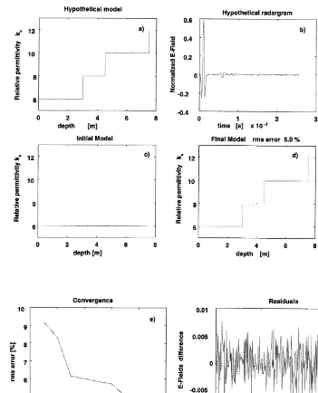
First, we consider the case of a permittivity radargram and its corresponding permittivity es-timation. The process is summarized in Fig. 2. The case is associated to a four-layer soil model
Ž .
with permittivity variations Fig. 2a and uni-form conductivity and permeability. The hypo-thetical radargram was contaminated with a level of random noise of 5% and is shown in Fig. 2b. In the estimation process, the initial model has six layers with the following parameters: ´is
6´0, sis0.001 Srm, mism0 for is1 to 6 ŽFig. 2c . The conductivity and permeability. profiles are kept fixed to their original and uniform values. The permittivity of each of the six layers is allowed to vary from iteration to iteration until they converge to the model shown
in Fig. 2d. The history of the process on its way to convergence is shown in Fig. 2e. In the present case, the final model is obtained in nine iterations with a rms errors5.0%. The differ-ence between the estimated and hypothetical radargrams is shown in Fig. 2f. The fact that the estimated and the hypothetical models are al-most identical, and that the residuals are of the level of the added noise illustrates the effective-ness of the approach for the case of permittivity estimation.
3.2. Estimation of conductiÕity
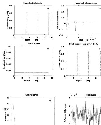
We now consider the case of conductivity estimation using as data a conductivity radar-gram. The process is summarized in Fig. 3. The model in this case is made up of three conduc-tive thin layers embedded in a relaconduc-tively less
Ž .
conductive medium of 0.001 Srm Fig. 3a . The hypothetical radargram was contaminated with a level of random noise of 2% and is shown in Fig. 3b. The model is uniform in
Ž . Ž
permittivity ´s10´0 and permeability ms
.
m0 . These quantities were not allowed to change in the inversion process, only the conductivities of the thin and thick layers took part in the optimization. The initial model has seven layers with the following properties ´is10´0, sis
0.001 Srm, mism0 for is1 to 7 Fig. 3c; the estimating process tends to recover the model with an rms errors2.1% after relative few iterations. The rather sharp drop in rms error in the very first iteration is something that called
Ž .
our attention Fig. 3e . We believe that this is an indication that the inverse problem for conduc-tivity is nearly linear when it is posed in terms of isolated thin layers. This is understandable from a physical point of view considering that there is almost no change in velocity when going from the initial to the final model.
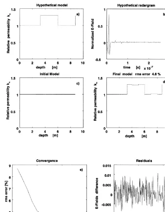
3.3. Estimation of permeability
Ž . Ž .
Fig. 2. Permittivity estimation from a permittivity radargram. a Hypothetical model with permittivity variations. b
Ž . Ž .
Hypothetical radargram used as data with 5% random noise added. c Initial model in the inversion process. d Final
Ž . Ž .
estimated model with its rms error. e History of the process on its way to convergence. f Difference between the estimated and the hypothetical radargrams.
radargram. The process begins by considering as data the radargram shown in Fig. 4b, which in this case has a noise level of 5% and ends with the estimated model represented in Fig. 4d. In this case, the initial model is made up of 10
layers with the following parameters: ´is2´0,
Ž . Ž .
Fig. 3. Conductivity estimation from a conductivity radargram. a Hypothetical model with conductivity variations. b
Ž .
Synthetic radargram with 2% random noise added. c Conductive halfspace used as starting model in the inversion process.
Ž .d Recovered model with its corresponding rms error. e History of convergence. Notice that the process converges fasterŽ .
Ž .
than for the case of permittivity Fig. 2 . This happens especially around the first iterations and indicates that the problem is
Ž .
nearly linear for conductivity. f Difference between the estimated and the hypothetical radargrams.
3.4. Cross-estimation
We have considered so far the estimation of a given property from radargrams computed using the same property. We have done this for per-mittivity, permeability and conductivity. Results
demon-Ž . Ž .
Fig. 4. Permeability estimation from a permeability radargram. a Hypothetical model with permeability variations. b
Ž . Ž .
Hypothetical radargram with 5% random noise added. c Halfspace used as starting model in the inversion process. d
Ž . Ž .
Final permeability model with its rms error. e History of convergence. f E-fields difference between the radargram of the final model and the hypothetical radargram.
strate that the method can handle discontinuities at arbitrary depths. Nevertheless, the above-tests suffice for a confident application of the method to the second objective of the work, which is to demonstrate that a given radargram can be inter-preted in terms of any of the three
electromag-netics properties. This is the aim of the exam-ples discussed below.
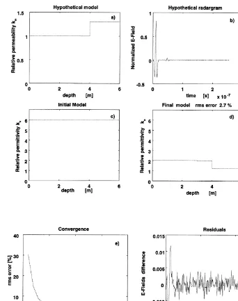
disconti-Ž .
Fig. 5. Permittivity estimation from a permeability radargram. a Hypothetical two-layer model that is uniform in
Ž .
conductivity and permittivity but not in permeability. b Hypothetical radargram used as data with 2% random noise added.
Ž .c Dielectric halfspace used as starting model in the inversion process. d Final permittivity estimated model with itsŽ .
corresponding rms error. The reflection in the radargram is due to the discontinuity in permeability but it is interpreted as a
Ž . Ž .
discontinuity in permittivity. e History of the process on its way to convergence. f Residuals.
nuity as shown in Fig. 5a. Instead of attempting to recover the jump in permeability, we con-sider that the corresponding reflection is due to a discontinuity in permittivity, and proceed to estimate the equivalent model which is shown in Fig. 5d. The initial model, with five possible
discontinuities, consisted of six layers with the following parameters: ´is6´0, sis0.001 Srm and mism0, is1 to 6 Fig. 5c. The rms errors2.7% was arrived at in 17 iterations.
Ž .
Fig. 6. Permeability estimation from a permittivity radargram. a Hypothetical model that is uniform in conductivity and
Ž . Ž .
permeability but not in permittivity. b Hypothetical radargram used as data with 2% random noise added. c Halfspace
Ž .
used as starting model in the inversion process. d Final permeability model with its rms estimation error. The reflection in
Ž .
the radargram is due to the discontinuity in permittivity but it is interpreted as a discontinuity in permeability. e History of
Ž .
convergence. f E-fields difference between the radargram of the final model and the hypothetical radargram.
considering a discontinuity in permittivity only and it is interpreted in terms of permeability. The estimated model is shown in Fig. 6d. In this case, the initial model consisted of 10 layers with the following parameters: ´is4´0, sis
0.0004 Srm, and mism0 for is1 to 10 Fig.
6c. The rms errors2.4% was reached in 10 iterations. The hypothetical radargram was con-taminated with a level of noise of 2%.
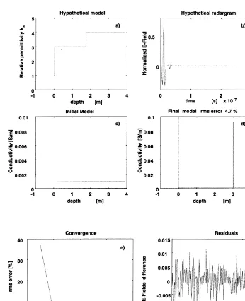
in Fig. 7. In this case, the equivalent of one permittivity discontinuity is a double discontinu-ity in conductivdiscontinu-ity or thin conductive layer. The hypothetical model is shown in Fig. 7a. We
explain the data with a model containing two thin conductive layers, one right on the surface and the other at depth. The first accounts for the surface discontinuity and the other for the
per-Ž .
Fig. 7. Conductivity estimation from a permittivity radargram. a Hypothetical model that is uniform in conductivity and
Ž . Ž .
permeability but not in permittivity. b Synthetic radargram with 5% random noise added. c Conductivity halfspace used
Ž .
as starting model in the iterative inversion process. d Final estimated model with its corresponding rms estimation error. The reflections in the radargram, including the first reflection right from the surface, are due to the discontinuities in permittivity. In this case, both reflections are interpreted in terms of conductivity variations. The equivalent model consists of two thin conductive layers, one right on the surface to account for the contrast in permittivity between air and soil, and the
Ž . Ž .
mittivity boundary at depth. The initial model consisted of seven layers with the following parameters: ´is6´0, sis0.001 Srm, and mi
sm0 for is1 to 7 Fig. 7c. The rms errors
4.7% was reached in eight iterations. The hypo-thetical radargram was contaminated in this case with a level of noise of 5%.
4. Conclusion and discussion
At first sight, the results presented in this paper might appear as pessimistic, in the sense that they point out the impossibility of recover-ing jointly the three electromagnetic properties from GPR data. Before reaching for this conclu-sion, one must take into consideration that our approach to the problem is perhaps the simplest possible. It is true that for a plane wave with horizontal fields this impossibility exists, as demonstrated by the present work. The possibil-ity of differentiation must come from a further complication of the physical model, by includ-ing for instance frequency dependent properties on one hand, or by considering vertical electric fields on the other. This may change the picture drastically. As they stand, the present results should be seen as an ideal limit case that di-rectly points out to the impossibility of differen-tiation.
Acknowledgements
The first author wishes to express his grati-tude to the CONACYT, Facultad de Ingenierıa
´
de la UNAM, CICESE and the Gran
Frater-Ž .
nidad Universal, Lınea Solar, A.C. REDGFU
´
for the support during the development of this project, and to the reviewers of this paper.References
Esparza, F.J., Gomez-Trevino, E., 1996. Inversion of mag-´ ˜
netotelluric soundings using a new integral forms of the induction equation. Geophys. J. Int. 127, 452–460. Esparza, F.J., Gomez-Trevino, E., 1997. 1-D inversion of´ ˜
resistivity and induced polarization data for the least
Ž .
number of layers. Geophysics 62 6 , 1724–1729. Gill, P.E., Hammarling, S.J., Murray, W., Saunders, M.A.,
Ž
Wright, M.H., 1986. User’s guide for LSSOL Version
.
1.0 : a FORTRAN package for constrained linear least squares and convex quadratic programming, Technical Report Sol 86-1. Department of Operations Research, Standford University, CA, USA, 38 pp.
Gomez-Trevino, E., 1987. Nonlinear integral equations for´ ˜
Ž .
electromagnetic inverse problems. Geophysics 52 9 , 1297–1302.
Gomez-Trevino, E., 1999. Reworking Maxwell’s equations´ ˜
in search of alternative approaches for inversion. Sub-mitted to Geophysical Journal International.
Lazaro-Mancilla, O., Gomez-Trevino, E., 1996. Synthetic´ ´ ˜
radargrams from electrical conductivity and magnetic permeability variations. J. Appl. Geophys. 34, 283–290. Levenberg, K., 1944. A method for the solution of certain nonlinear problems in least squares. Q. Appl. Math. 2, 164–168.
Mardquardt, D.W., 1963. An algorithm for least squares estimation of nonlinear parameters. SIAM J. 11, 431– 441.
McGillivray, P.R., Oldenburg, D.W., 1990. Methods for calculating Frechet derivatives and sensitivities for the´
nonlinear inverse problem: a comparative study. Geo-phys. Prospect. 38, 499–524.