www.elsevier.com/locate/econedurev
Schooling of girls and boys in a West African country: the
effects of parental education, income, and household
structure
Peter Glick
*, David E. Sahn
Cornell University, 3M28 Van Rensselaer Hall, Ithaca, NY 14853, USA
Received 4 June 1997; accepted 15 October 1998
Abstract
In this paper we investigate gender differences in the determinants of several schooling indicators—grade attainment, current enrollment, and withdrawal from school—in a poor urban environment in West Africa, using ordered and binary probit models incorporating household-level random effects. Increases in household income lead to greater investments in girls’ schooling but have no significant impact on schooling of boys. Improvements in father’s education raises the schooling of both sons and daughters (favoring the latter) but mother’s education has significant impact only on daught-ers’ schooling; these estimates are suggestive of differences in maternal and paternal preferences for schooling daughters relative to sons. Domestic responsibilities, represented for example by the number of very young siblings, impinge strongly on girls’ education but not on boys’. Policies such as subsidized childcare that reduce the opportunity cost of girls’ time in the home may therefore increase their ability to get an education. JEL 015, I211999 Elsevier Science Ltd. All rights reserved.
Keywords:Economic development; Human capital
1. Introduction
Low levels of human capital are widely considered to be a major impediment to economic growth and the elimination of poverty in sub-Saharan Africa. Recent studies of several African countries document the exist-ence of returns in the labor market to investments in edu-cation for both men and women.1Researchers and
pol-* Corresponding author. Fax: 1 1-607-255-0178; e-mail: [email protected]
1Studies estimating earnings functions disaggregated by gen-der and including appropriate controls for selection into the labor force or into particular sectors include those by Vijverberg (1993); Glick and Sahn (1997); and Appleton, Hoddinott, Krishnan and Max (1995). These studies generally find signifi-cant schooling impacts on both male and female earnings. It has been argued, however, that private returns to primary edu-cation in Africa have fallen in recent years (see Appleton et al., 1995; Knight, Sabot & Hovey, 1992).
0272-7757/99/$ - see front matter1999 Elsevier Science Ltd. All rights reserved. PII: S 0 2 7 2 - 7 7 5 7 ( 9 9 ) 0 0 0 2 9 - 1
icy-makers have increasingly recognized the benefits in particular to expanding girls’ access to schooling. Improvements in women’s education will help to elimin-ate gender inequalities in employment opportunities and earnings and will also have important non-market bene-fits such as better child nutrition and lower fertility (Strauss & Thomas, 1995). However, despite dramatic increases in both male and female enrollments in the first few decades after independence, girls’ schooling in African countries still lags behind that of boys at all lev-els and particularly at post-primary levlev-els (World Bank, 1988).
enrollment rates remain below 40%, however—among the lowest in the world (World Bank, 1995). In addition, in spite of a commitment to improving girls’ access to schooling, the ratio of female to male primary students in 1993 was only 44%. This gender disparity in enrollments increases sharply with education level: girls represent only 25% of lower secondary students, 20% of upper secondary students, and just 6% of university students. Thus gender in Guinea is an important determinant both of attending school at all and of the level of schooling achieved.
In light of the benefits to investments in education, it is important to identify the factors underlying household decisions regarding the education of children, and especially decisions about girls’ schooling. The edu-cation of parents has been found in many studies to be one of the most important determinants of child school-ing. Of particular interest in the West African context, where incomplete pooling of household resources appears to be the norm and preferences of husbands and wives may diverge sharply,2 is whether maternal and paternal schooling have equivalent effects on the cation of boys and girls. It might be expected that edu-cated women have both strong preferences for schooling their daughters (preferences which may not be shared by their spouses) and the ability to ensure that household resources are allocated for this purpose. If as a conse-quence of these factors a mother’s education has a greater impact on girls’ schooling than on boys’, there would be a further rationale for public investments in female schooling: the intergenerational effects of such investments will lead in the future to even greater reductions in the gender gap in schooling and ultimately, in earnings.
Boys and girls may also differ with respect to the ways in which household structure, in particular the presence of young children, impinges upon their ability to acquire an education by affecting the burden of household responsibilities. These responsibilities are likely to be imposed on girls more than boys. If this is the case, then policies (for example, subsidized childcare) that reduce the dependence of households on the domestic labor of girls may increase girls’ enrollments, thus also helping to close the gender gap in schooling.
Research on the household determinants of schooling is quite sparse for sub-Saharan Africa, owing in part to
2There is a sizable anthropological literature for Africa, and West Africa specifically, indicating that men and women within households do not pool income or make expenditure decisions jointly. See, for example, Fapohunda (1988), Munachonga (1988), and Guyer and Peters (1987) and references therein. Complementing these studies is the econometric analysis of household expenditures in Coˆte d’Ivoire by Hoddinott and Had-dad (1995), who find that expenditure patterns differ depending on the share of total family income earned by women.
the shortage until recently of comprehensive household level data sets from the region.3 This study examines schooling choices using household survey data from Conakry, the capital and largest urban area of Guinea. We focus on the impact of parental education, household structure, and income on the schooling of boys and girls. Several schooling outcomes are examined in the empiri-cal work in this paper: years of schooling or grade attain-ment; current enrollment status; and leaving school. We focus on multiple schooling indicators instead of a single one, such as current enrollment, for two reasons. First, each of the three illuminates a different aspect of school-ing choice and thus is of interest in its own right. Second, as described in detail below, each has both advantages and disadvantages, the latter largely reflecting limits in the available data. Since each approach is imperfect, checking for consistency of results with regard to key variables provides a useful informal test of the robust-ness of the findings.
The remainder of this paper is organized as follows. Section 2 outlines the conceptual framework underlying the empirical work and Section 3 discusses the econo-metric methodology. The dataset is described and some descriptive results are discussed in Section 4. The econo-metric results are presented in Section 5. The paper con-cludes in Section 6 with a discussion of policy impli-cations of the results.
2. Conceptual framework
Underlying the empirical analysis in this paper is a conceptual model of parental or household decision-making regarding investments in the education of boys and girls.4 We assume for the time being a “unitary”
3Much of what has been done has used the World Bank’s Living Standards Measurement Survey data from Ghana and Coˆte d’Ivoire (see, e.g. Tansel, 1997; Glewwe & Jacoby, 1994). An earlier analysis by Chernichovsky (1985) focused on chil-dren in rural Botswana.
model of the household such that preferences of the mother and father are identical, or that if they are not, the household nevertheless acts as if it were maximizing a single utility function (which would occur if the prefer-ences of only one of the parents counted). Parents are assumed to live for two periods. For a household con-sisting of a mother, father,mdaughters andnsons,5 par-ental preferences are assumed to be represented by a util-ity function
U5U(Ct,Ct11,Sd1,...,Sdm,Ss1,...,Ssn) (1)
whereCtandCt+1denote household (parental) consump-tion in the first and second periods andSdiandSsjdenote the education of theith daughter andjth son. The second period consumption of the parents depends through remittances on their children’s income, denoted byYdit+1 andYsjt+1. Children’s income or wealth in the second per-iod depends in turn on the level of schooling attained in the first period as well as on child-specific variables Z such as sex and natural ability, e.g.Ydit+15Ydit+1(Sdi,Zdi) for theith daughter. Transfers from child to parent in the second period will vary by child characteristics through their effects both on income and on remittance propen-sities; in particular, for cultural reasons daughters may remit a smaller portion of their incomes than sons. Thus we have for second period parental consumption:
Ct115Ct11(Yd1t11,...,Ydmt11,Ys1t11,...,Ysnt11; (2)
Zd1,...,Zdm,Zs1,...,Zsn)
Parents are assumed to care about the wealth or income of their children because of the benefits to their own future consumption through remittances, but they may, of course, also be altruistic and care about their children’s future welfare. In this case children’s wealth would appear as separate arguments in the utility func-tion. In either case the nature of schooling as an invest-ment is clear: greater education expenditures, financed through reductions in current consumptionCtor though borrowing, result in higher levels of income for the chil-dren and consumption for the parents in the second per-iod.6The education of the children also enters into the
presented below, and the fact that enrollments of fostered-in children are lower than those of children living with parents, suggest that even within extended families, the characteristics of the nuclear family retain substantial importance as school-ing determinants.
5The number of children is taken as predetermined rather than as a choice variable, an assumption that raises concerns for the estimation. These are addressed below.
6For girls in particular there may also be significant non-pecuniary returns to education investments not represented in this simplified model, such as improved child health, which par-ents may also value.
parental utility function Eq. (1) directly, since parents may also enjoy having educated children. The simplified framework above thus brings out the nature of education as both an investment good and a consumption good.7
Parents in the first period face a full income constraint:
F5V1Tmwm1Tfwf1
O
m
1
Tdiw*d1
O
n
1
Tsjw*s (3)
whereVis unearned income,Tm,Tf,Tdi, andTsjare the total times available to the mother, father, the ith daughter and thejth son; andwm,wf,w*dandw*sare their respective wage rates. The contribution of children’s time to household full income should be emphasized. Children in developing countries typically make pro-ductive contributions to household welfare through work in the home, for example by caring for younger children, or in the family farm or business. Where there is a mar-ket for child labor they can also work for others. If such a market exists,wdandwsare the market wage rates for girls’ and boys’ labor; otherwise they represent implicit prices of time determined endogenously by both the demand for household goods and services that use chil-dren’s labor and the home production technology (“*” is used to indicate that these are potentially endogenous variables).
Assuming for convenience that the time of children is divided between such work and schooling and that of parents between work and leisure, the full income con-straint can be expressed in terms of expenditures on leis-ure, goods, and schooling:
F5V1Lmwm1Lfwf1PcCt1
O
m
1
(PsSdi (4)
1w*
dTSdi)1
O
n1
(PsSsj1w*sTSsj)
whereLmandLfare the leisure of mother and father;Ps are direct costs per child of schooling; and Tdi and Tsj represent the time of the ith daughter and jth son, respectively, devoted to schooling. Regarding the com-position ofPs, direct schooling costs in Guinea do not generally include tuition since virtually all primary stu-dents and the great majority of stustu-dents in higher levels attend public schools, which are free.8 However, other
7The latter aspect of schooling is emphasized in household production models incorporating child quantity and quality (Becker & Lewis, 1973; Willis, 1973). In this framework, par-ents derive utility from both the number of children they have and their quality, an important dimension of which is their schooling, and both quantity and quality are choice variables.
direct private costs such as books, uniforms, and trans-portation appear to be considerable: they were cited in interviews of parents and students as a major barrier to school attendance (World Bank, 1995). w*
dTSdi and
w*
sTSsj, the hours of the daughter and son spent in school
or schoolwork multiplied by the price of their time, rep-resent the foregone contributions to household (or market) production of having the daughter and son attend school. Each term in brackets combines this opportunity cost with direct costs PsSdi orPsSsjand thus represents the total cost of schooling for each boy or girl.
Parents maximize utility subject to the full income constraint and the constraints relating earnings to school-ing and parental consumption to child earnschool-ings, resultschool-ing in reduced-form demand equations for boys’ and girls’ quantity of schooling (as well as for other goods and leisure) as functions of all prices and wages, vectors of individual factors Zand household and community
fac-tors H, and maternal and paternal educationSm andSf:
Sdi5Sdi(wm,wf,V,Pc,Ps,Sm,Sf,Zdi,...,Zdm,Zs1,...,Zsn,H) (5)
Ssj5Ssj(wm,wf,V,Pc,Ps,Sm,Sf,Zdi,...,Zdm,Zs1,...,Zsn,H)
As indicated in the introduction, parents may have dif-ferent preference orderings, including difdif-ferent prefer-ences for schooling, in which case the assumption of a unique parental utility function such as that in Eq. (1) is invalid. A variety of theoretical models of the household that incorporate differing preferences of household mem-bers (e.g. husbands and wives, mothers and fathers) have been developed and are referred to as “collective” house-hold models. We briefly describe the approach here rather than present it formally because the reduced-form demand functions for schooling derived in such a frame-work are (for our dataset) identical to those just derived within the common preference framework. Collective models posit separate utility functions for the husband and wife. When preferences differ there must be some mechanism for determining how to allocate household resources; the most common assumption is that the household engages in a cooperative bargaining game leading to Nash equilibrium demands for commodities (McElroy & Horney, 1981). Each partner’s power in bar-gaining is a function of the income under his or her direct control and, ultimately, of the utility he or she would be able to achieve outside of the marriage—the “threat point”—since this represents the fallback position.9The
9That is, with a stronger fallback position, a partner can thre-aten more credibly to dissolve the partnership if allocations are not sufficiently in line with her or his preferences. More realisti-cally for smaller allocation decisions, the partner can threaten to retreat to a non-cooperative solution, where budgets are com-pletely separate, while maintaining the partnership (see Alder-man, Chiappori, Haddad, Hoddintot & Kanbur, 1995).
threat point, hence bargaining power, is a function of “extrahousehold environmental factors” (McElroy, 1990) that affect opportunities outside the partnership. These include unearned income accruing to the individual, sex-and education-specific wage sex-and employment rates, the legal framework (as regards, for example, child-support), and the partner’s possibilities for remarriage or financial support from relatives.
Reduced-form demand equations for schooling
derived from a bargaining framework would include such factors in addition to those already in Eq. (5). Test-ing the unitary household model against the more general collective model essentially involves testing for the sig-nificance of extrahousehold environmental variables that would not affect schooling under common preferences. A variant of this approach involves comparing the effects of unearned (that is, exogenous) income received by each spouse.10Unfortunately, our dataset lacks information on (or variation in) these factors, so we cannot augment our reduced-form equations to conduct such a test. Still, the notion of non-unified preferences and bargaining over resources within the household has substantial appeal in the present context and will be helpful in interpreting some of the empirical results of this study.
The direction of the effects of a number of the vari-ables in the schooling demand function can be predicted from theory.11In particular, factors that raise perceived returns or lower the costs of education will raise invest-ments in education. The schooling of the parents (Smand Sf) is one such factor and is expected to be positively associated with children’s schooling. Educated parents are more able to assist in their children’s learning, raising the returns relative to less educated parents, and are also
10The unitary model assumes that income is completely pooled so the source of income should not matter for allo-cations; hence common preferences are rejected if the effects of husband’s and wife’s unearned income differ. The equality of male and female income effects has been rejected for out-comes such as own labor supply (Schultz, 1990), child health (Thomas, 1990), and household expenditure shares on health, education and housing (Thomas, 1993). Rao and Greene (1991) find that a woman’s bargaining power, proxied by female employment rates and sex ratios (reflecting re-marriage possibilities) significantly affects fertility decisions. Handa (1996) uses female headship, treated as endogenous, as a proxy for maternal bargaining power within the household in school-ing demand equations and finds a positive effect of this variable on schooling. However, some of the exclusion restrictions imposed for identification of the structural schooling equations are questionable; it is assumed, for example, that age and edu-cation of the head has no direct impact on child schooling.
more likely to recognize the benefits of schooling. Posi-tive parental schooling impacts are also expected from a schooling as a consumption good perspective, since bet-ter-educated parents are likely to enjoy educated children more than less-educated parents; thus mother and father education will act as taste-shifters in the schooling demand functions.
Like parents’ education, household income will, under plausible assumptions for developing countries, posi-tively influence the demand for children’s education. Poor households may be unable to afford the direct or indirect costs of schooling and be constrained in their ability to borrow to cover the costs. Since wealthier households are likely to be able to pay for schooling out of current income or savings (and have easier access to credit), children from such households are expected to be more likely to enroll and to stay in school longer. Income will also have a positive effect on schooling if education is a “normal” consumption good.12
Gender differences in schooling—namely, greater schooling for boys—can come about because the returns to educating boys are greater than for girls or because the costs are lower, or because parents simply prefer edu-cating sons.13With regard to returns, if women are dis-criminated against in the labor market in terms of access to employment or in earnings, the monetary benefits to
12Another potentially important determinant of the demand for schooling is school (or teacher) quality, which affects the labor market productivity benefits of schooling and possibly, through impacts on grade repetition, the costs of attaining a given grade level. Data on school quality are not available for this study; even if they were, it is uncertain whether sufficient cross-sectional variation would exist within the region surveyed (urban and peri-urban Conakry) to enable estimation of the effects of changes in quality on schooling demand. The same considerations apply to direct costs of schooling (books, uni-forms, etc.). Thus we focus on the socio-economic character-istics of households.
13More precisely, if direct impacts on parental utility of child schooling are ignored, so that parents care only to maximize their consumption, the first order conditions of the model imply that the relative marginal effects of female and male education on parents’ second period consumption will equal the relative marginal costs of educating girls and boys (the ratio of opport-unity costs if direct costs are zero), i.e.
∂Ct11/∂Sd
∂Ct11/∂Ss
5w
* d w* s
With diminishing marginal second period consumption returns to schooling, a reduction in the marginal benefit to schooling girls relative to boys (the ratio to the left of the equality) implies a lower optimal level of investment in girls’ education. Similarly, an increase in the relative opportunity cost for girls implies a reduction in girls’ schooling relative to that of boys.
investing in their education will be lower than for boys.14 As noted, there may be substantial returns to female schooling in non-market production, but parents may not be aware of these non-pecuniary benefits or may value them less than monetary ones. Even if educated girls go on to work and receive earnings on a par with men, income remittances to parents from married adult daugh-ters, who join their spouses’ families, may be lower than from adult sons. Finally, the returns to parents from edu-cating girls could be low because the quality of the schooling that girls receive is poor, reflecting school and teacher attitudes or interruptions in attendance or school-work resulting from girls’ household obligations.
The last factor mentioned points to the possibility that the opportunity cost of educating girls is higher than for boys. Girls in developing countries are typically called on to perform more household work than boys, reflecting cultural or social attitudes toward the proper economic roles of women and girls. Given these attitudes, the mar-ginal cost of girls’ time will be higher than boys’ (w*
d>w*s) and consequently the demand for their school-ing will be lower.15,16 For the same reasons, it would
14More precisely, the incremental effects of schooling on expected earnings, determined by employment entry prob-abilities and wages, must be lower for women for this to be the case. Previous work on Conakry using this dataset (Glick & Sahn, 1997) was unable to reject the hypothesis that the returns to schooling (in either wage employment or self-employment) were the same for men and women, but did find a non-linear effect of schooling on women’s employment probabilities: rela-tive to no education, the likelihood of working fell with primary education and rose with secondary schooling and college (levels which very few women in Guinea have attained). There appear to be relatively few opportunities outside of small-scale self-employment for women with just a primary education.
15This may not be the case if there is also a strong demand for boys’ labor on the family farm or in a family enterprise, but neither of these possibilities is very relevant in the current context. Agriculture is not a major activity in the urban and peri-urban setting of this study, and participation of adolescent boys (and girls) in household enterprises (and for that matter, in wage employment) appears to be quite low (Glick & Sahn, 1997).
also be expected that certain changes in household struc-ture will affect girls’ schooling more strongly than boys’. An increase (assumed exogenous) in the number of very young children, for example, may raise the demand for the labor of girls in childcare in the home. Given the time constraint, this will reduce their schooling relative to that of boys. By the same logic, additional older sib-lings or adult women may reduce the opportunity cost of a girl’s time by providing substitutes for household work or through economies of scale in household pro-duction, thereby raising the likelihood of enrollment or the average level of schooling among girls in the house-hold.17In the empirical work, we do not attempt to esti-mate endogenous shadow prices of time for girls and boys. Instead, the reduced-form schooling demand func-tions include family composition and other household factors (represented by H in Eq. (5)) that are expected to influence, possibly differentially by gender, the value of children’s time.
Would the collective household model with individual preferences generate any different expectations about the impacts of the factors discussed above on girls’ and boys’ schooling? The model predicts that factors that raise the bargaining power of the wife should increase allocations to goods she prefers. The mother’s education stands out as one such factor for which the dataset pro-vides information. Women with more schooling are able to earn more, improving their fallback position and (if they are actually working) the level of income under their direct control. Thus, if women value the schooling of their children more than men do, maternal schooling will have a stronger impact than paternal schooling on children’s education. Further, mothers may prefer to allo-cate resources (including for human capital) to daughters while fathers prefer sons, as suggested by evidence for
work, in preparation for their future likely roles as homemakers. As a result of this initial specialization and investment, girl’s home productivity will be higher than boys in later periods, hence their opportunity costs will be higher. This is akin to the “efficient specialization” hypothesis of Becker (1981). Thus the gender difference in the price of time is a manifestation of lower returns to schooling for girls, not parental preferences.
17Note that this conflicts with a major implication of the quantity–quality model described in note 7: that child quantity and quality (average schooling) should be inversely related. An inverse relationship exists because having more children raises the cost of providing a given amount of education resources to each child, and conversely, a higher level of quality raises the implicit price of child quantity. However, in a context where child work is important, so that the cost of schooling includes the opportunity cost of foregone labor in the home or family farm/enterprise, the relation of the number of children to aver-age educational investment is less obvious. As noted in the text, increases in the number of children in particular age or sex categories can lower the marginal value of an individual child’s time, encouraging school investments.
child height in the US, Ghana and Brazil presented in Thomas (1992). Then increases in mother’s schooling would have a larger beneficial effect on daughters’ edu-cation than on sons’, and father’s schooling would favor sons’ education. The former is particularly plausible because the mother’s bargaining power and her prefer-ences for daughters’ schooling are both likely to rise with her own education.
Note, however, that these relationships of maternal and child schooling are also compatible with unified household preferences. For example, a larger maternal education impact on girls’ education than boys’ may reflect maternal preferences for schooling girls in a bar-gaining framework or that households in which the mother has an education also have strongcommon pref-erences for girls’ schooling. The latter will arise through marital sorting if men who choose educated wives also want educated daughters (or if educated women choose spouses who also have a preference for educating daughters), resulting in heterogeneity in preferences between households rather than within them. The prob-lem, as stated above, is that the dataset does not provide a measure of individual bargaining positions that would not also be a determinant of schooling under common household preferences.18
3. Empirical approaches
3.1. Years of schooling
The first schooling outcome we investigate, years of schooling or grade attainment, is an indicator of the cumulative investment in an individual’s education. We use an ordered probit model to estimate the determinants of years of schooling. This approach allows us to incor-porate several features of the data that simpler alterna-tives, such as ordinary least squares, cannot. For example, OLS assumes a continuous distribution for the dependent variable, grade level. Grade attainment, how-ever, represents the outcome of a series of ordered dis-crete choices—whether to go on to the next grade or withdraw from school. Also, the distribution of years of schooling is usually not normal around the mean. Typi-cally it is bimodal or even trimodal, with peaks
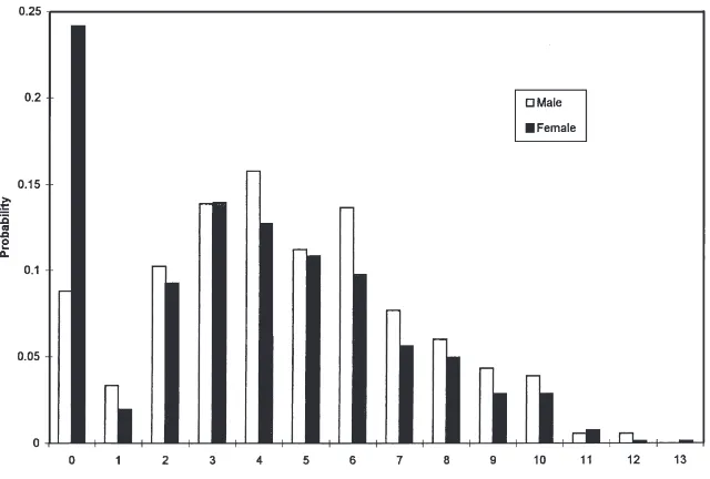
Fig. 1. Males and females aged 10–18: distribution of years of schooling.
resenting completion of specific levels, e.g. secondary school. In our sample, as shown in Fig. 1, the distribution of years of school is not punctuated by sharp spikes but nevertheless bears little resemblance to a normal distri-bution. For girls especially many observations cluster at zero (no schooling); for both boys and girls there are sharp drops following 6th grade (completed primary) and 10th grade (completed lower secondary).
A third feature of the data is sample censoring. For children who are still enrolled, the current grade level does not necessarily represent their final grade attain-ment; all that is known is that they will ultimately have completed at least their last grade. The data on schooling for these observations, in other words, are right-cen-sored. Not taking this censoring into account—that is, considering the education of such individuals to be ident-ical to those who have ended their schooling at that grade—will result in biased estimates of the effects of the regressors on true (potential) grade attainment.19
The ordered probit model treats grade attainment as the outcome of ordered discrete choices and does not assume a normal distribution for the dependent variable. The model can also be extended to allow for right-cen-soring of years of schooling. Although completed
19The censoring problem can be eliminated by restricting the sample to cohorts old enough to have completed their schooling by the time of the survey, but this restricts the focus to an older group in a context where the determinants of schooling may have changed over time. In any case, as described in the next section, data on parental backgrounds as well as relevant house-hold characteristics are unavailable for adults not still residing with their parents.
schooling for children who are still in school is not known, it is known that the final grade attained will be at least as high as the last grade. This information is incorporated into the likelihood function of the model, making it possible to calculate unbiased estimates of pro-jected completed schooling of an individual of given characteristics.20
A further consideration for the estimation is that the residual terms are unlikely to be independent, reflecting the fact that more than one child from the same house-hold may appear in the estimating sample. Children in the same household are likely to share unmeasured (by the researcher) traits that make them more or less able to perform well in school, affecting their demand for schooling in a similar way. Alternatively, households may be heterogeneous with respect to unobserved prefer-ences for education. In either case, the error terms for children from the same household will be correlated through a common family-level component, and if ignored this lack of independence may result in substan-tially underestimated standard errors. We allow for such correlations in the model through a random effects or variance component structure for the residuals; that is, the errors of the index functions for schooling in the ordered probit formulation are assumed to consist of a common household heterogeneity component and an idiosyncratic individual error. The estimation procedure used is that suggested by Butler and Moffit (1982) for the random effects binary probit model. Details of the
likelihood function and estimation of the random effects ordered probit model with censoring are presented in Appendix A.
We estimate separate ordered probit models of years of schooling for boys and girls aged 10–18. The reason for choosing age 10 as the lower end of the range is that delayed primary enrollment appears to be common in Conakry, so that some children who are, say, 8 or 9 and who have never been enrolled may yet enter. For these children it would clearly be inappropriate to assign a value of zero for grade attainment. By including only children 10 and over, we can be reasonably sure that those who have not yet enrolled will never enroll and can be assigned zero years of schooling. The choice of age 18 as the upper end of the range is dictated in part by the desire to minimize selectivity problems caused by older children being absent from the household, an issue we discuss in detail below.
3.2. Current enrollment status
Next we estimate the determinants of school
enrollment status at the time of the survey. For assessing the effects of factors that are time-varying, analyzing the current enrollment decision has advantages over the analysis of cumulative schooling just outlined, since it allows us to relate current school choices to contempor-aneous aspects of the household such as income and household structure. The latter includes the presence of young siblings, whose arrival will likely alter the allo-cation of time among schooling, household work, and other uses.21On the other hand, a disadvantage of the current enrollment approach is that (unlike the ordered probit model of grade attainment) it implicitly assumes that the current enrollment decision is independent of the choices made in previous years; that is, it ignores the cumulative nature of schooling decisions. This is gener-ally not a very plausible assumption: with the exception of younger children just beginning their schooling, a child is more likely to be in school today if he or she has been previously enrolled than if she has never attended
21If parents determine both the number and spacing of chil-dren and future investments in their schooling at the start of childbearing or marriage, events such as a recent birth are anticipated and reflected in the cumulative schooling of older siblings. It would then suffice only to look at the ordered probit models of grade attainment (but excluding sibling covariates from the equation, since they would clearly be endogenous). However, this assumes a very high level of planning on the part of parents as well as an absence of uncertainty, both of which are unlikely in a poorly educated population with limited access to contraceptives. The issue of the endogeneity of children is considered further below.
school.22 Current enrollment decisions are estimated using a binary probit, with the dependent variable taking the value of 1 if the child is currently attending school and zero otherwise. As with the ordered probits, we allow for intrahousehold correlations in the disturbances. The model we estimate is therefore the random effects binary probit model of Butler and Moffit (1982).
3.3. Leaving school
Our third approach is somewhat novel and focuses on a transition in schooling status: leaving school in the past 5 years. The ordered probit model of grade attainment implicitly also models the decision of when (i.e. after how many years of school) to withdraw. Here, however, we focus on the school departure decision within a spe-cific historical period. Since this period is recent (the last 5 years), our right-hand-side variables should fairly closely capture the circumstances relevant to the decision. The survey does not actually record the time since leaving school, so we impute it from the data using information on the ages of students currently in each grade. Years since leaving school is estimated as the individual’s current age minus the sex-specific median age of students currently enrolled in the last grade that the individual attended. Thus our dependent variable for withdrawing in the past 5 years, WITHDRAW, equals 1 if, for an individual who is no longer enrolled and who reportssyears of schooling, agei2medians,5, where ageiis the child’s age and mediansis the median age for grade s. It equals zero for individuals who are still enrolled. Individuals no longer in school but who com-pleted upper secondary school during the period are also assigned WITHDRAW50, while those who were never enrolled are not included in the sample.23Inferring recent
22This may reflect state dependence: attendance in periodt makes attendance int11 more likely because (among other possible reasons) the cumulative acquisition of skills is more efficient with continuous schooling than with off-and-on enrollment. An alternative explanation involves individual or household heterogeneity: children with a propensity for learning (or who have parents with a preference for schooling) will be more likely to be enrolled each year, regardless of the direct effect of attendance in one year on attendance in the next. These concepts are discussed in the context of female labor force par-ticipation in Heckman (1981).
school exit decisions in this way allows in a limited way for a dynamic analysis of schooling transitions using cross-section data. For example, a key demographic vari-able on the right-hand side is the number of siblings under 5, i.e. the number of brothers and sisters born (and surviving and remaining in the household) during the last 5 years. The analysis thus shows how school status is affected by “fertility shocks”, that is, additions to the family of young children (treated as exogenous) during the period.
The determinants of leaving school are estimated using random effects probit on the samples of boys and girls aged 15–18 who, using the method just described, are inferred to have been enrolled at the start of the per-iod. Note that because of the way the dependent variable is constructed, we are effectively analyzing behavior since age 10 for children currently 15, since 11 for those now 16, and so on. Since leaving school earlier than age 10 is rare, restricting the sample to children 15 and older is appropriate.24
4. Data and descriptive statistics
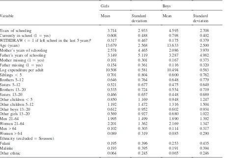
The data used in this study are taken from a survey of 1725 households conducted in Conakry in 1990. The survey contains detailed information on a wide range of socioeconomic factors such as education, labor force activity and earnings, assets, and health. Since the house-hold survey does not contain information on the charac-teristics of schools, the focus in this study is on the effects of household and individual factors on schooling. Our sample for analysis consists of boys and girls aged 10–18 living with at least one parent. Means and stan-dard deviations of the explanatory variables for boys and girls are given in Table 1.
We restrict the sample to children residing with a par-ent for two reasons. First, one of our primary concerns is the impact of parental education on child schooling,
24Since the sample consists of individuals inferred to have been in school 5 years earlier, the results must be regarded as being conditional on prior enrollment. Two other selection-related concerns should be noted. First, those who have recently left school and have also left the household are not recorded in the survey. Second, years since leaving school will, in general, be underestimated for children who started school late or repeated more grades than the typical child in their last grade, since these children would have been attending their last grade at a higher age than the median for the grade; the reverse is true for early starters and those who repeated less than the average. Overestimation of years since departure will cause some in the second group to be incorrectly dropped from the sample as non-recent (i.e. not within the last 5 years) school leavers, which might impart a bias to the estimates on the sample excluding them.
and the survey does not record the educational attain-ment of parents who do not live with their children (or of children who do not live with their parents). Second, for older children who no longer live with their parents, the characteristics of their present household, such as income and demographic composition, are not likely to be the relevant ones for determining the education out-comes of interest and may, in fact, be the outout-comes of prior schooling decisions: consider, for example, the case of a young man quitting school, going to work, and start-ing his own family. Given the cumulative nature of schooling decisions, the circumstances of the household in which the child was raised are more relevant, so for this reason as well we focus on children still living in the household of the parent or parents.
Although the choice of sample is necessary for these reasons, it involves a significant sample reduction. A siz-able percentage of children do not live with either parent and this ratio rises with age. For example, among all children in the sample age 13–18, 31% of girls and 44% of boys are living away from their parents. The data thus suggest that child fostering is an important phenomenon in Guinea, as elsewhere in West Africa (Ainsworth, 1992). In addition to fostering, older teenage children may move out of the households in which they were raised in order to marry, work, or attend school; early marriage of girls in particular is evident from our data. This raises the issue of selection bias in our estimates of the determinants of schooling, since households in which children are living with their parents may differ from other households in terms of unmeasured preferences or propensities for school (or children who leave may be different from children in the same household who stay).25The Conakry survey does not record the numbers
25The potential biases involved in restricting estimation of schooling functions to the sample of children living with a par-ent can be illustrated with the following elaboration of the Heckman selectivity model (Heckman, 1979; see also Pitt (1997) for a more detailed exposition of a model similar to the following). Assume that equations for the level of schooling (S) and selection into the sample of children observed to be living at home (H, an index function such thatH> 0 implies selection into the sample) take the following linear forms:
Si5xib11ub21ei5xib11ei
Hi5wig11ug21ui5wig11mi
Table 1
Boys and girls ages 10–18: variable means and standard deviations
Girls Boys
Variable Mean Standard Mean Standard
deviation deviation
Years of schooling 3.714 2.933 4.595 2.708
Currently in school (15yes) 0.608 0.488 0.798 0.402
WITHDRAW (51 if left school in the last 5 years)a 0.317 0.467 0.175 0.379
Age (years) 13.679 2.568 13.633 2.500
Mother’s years of schooling 2.574 4.465 2.086 3.970
Father’s years of schooling 3.149 5.119 3.287 4.982
Mother missing (15yes) 0.101 0.301 0.167 0.373
Father missing (15yes) 0.154 0.361 0.116 0.320
Log expenditure per adult 10.508 0.581 10.494 0.583
Siblings,5 0.701 0.804 0.600 0.762
Brothers 5–12 0.646 0.764 0.648 0.779
Sisters 5–12 0.521 0.677 0.475 0.649
Brothers 13–20 0.535 0.724 0.554 0.719
Sisters 13–20 0.466 0.657 0.448 0.689
Other children,5 0.850 1.169 0.948 1.247
Other children 5–12 1.192 1.472 1.316 1.504
Other boys 13–20 0.612 0.952 0.602 0.934
Other girls 13–20 0.569 0.927 0.680 1.022
Men 21–64 1.995 1.499 1.890 1.392
Women 21–64 2.201 1.362 2.169 1.347
Men > 64 0.102 0.303 0.114 0.317
Women > 64 0.089 0.319 0.085 0.290
Ethnicity (excluded5Soussou)
Fulani 0.195 0.396 0.253 0.435
Malinke 0.193 0.395 0.191 0.394
Other ethnic 0.064 0.245 0.065 0.246
aFor ages 15–18 and enrolled 5 years prior to survey (see text).
conditional on being in the sample of children living at home, substitute for corr(ei,mi) in the standard expression for a regression conditional on sample selection (Heckman, 1979) and take the derivative with respect toxk:
∂E(Si|Hi51)
∂(xk) 5bk2gkAib2g2s2u
whereAi5l2i 1wig1li,liis the inverse Mills ratio evaluated atwig1and is positive, as isAias long aswig1> 0 (as we would expect for positive selection into the home sample). The second term on the right-hand side represents the bias in the estimate ofbk, the effect of the change inxkon schooling, arising from sample selection. The direction of bias will depend on the signs of g2 and b2, the effects of schooling preference on sample selection and schooling, respectively, as well as on the sign of
gk, the coefficient ofxkin the selection equation. Sinceb2is positive, for a variable that increases the probability of selection into the with-parent sample (gk> 0), the estimate ofbkwill be biased downward ifg2is also positive, that is, if parents who (conditional on observed factors) prefer educated children are also more likely to keep them at home.
apparently came to Conakry after getting married, or to get married.26Thus girls who marry young and no longer live with their parents for the most part have not married out of Conakry households.
These rural to urban patterns of fostering, marriage, and migration in the data suggest that children and ado-lescents flow into households in Conakry (from which our estimating sample is drawn) far more than they flow out. Consequently, households (or more accurately, parents) in Conakry are “missing” fewer children as a result of out-fostering or early marriage than implied by the means for all children, which include children from non-sample rural households. This alleviates to some extent concerns over a large-scale selective elimination of observations from sample households.27On the other hand, selective rural–urban migration would imply that our randomly selected sample of households in Conakry, even with all children counted, is not representative of Guinea households overall. Given this possibility, it should be kept in mind that inferences regarding house-hold determinants of schooling are conditional on resi-dence in Conakry.28
26Among girls aged 14–18 in the Conakry sample who are married and living away from their parents, 81% were born outside of Conakry and the vast majority of these had arrived in Conakry in the previous 5 years. Their average age at the time of migration is high (14.2 years), suggesting that they were married when they migrated or came to get married rather than simply having migrated with their parents at a young age (in which case they would indeed have selected out of the sample of Conakry-resident households). Thus while there are many married girls in the sample under 18 not living at home, they appear by and large not to have come from sample households. As further evidence of this, we note that the ratio of boys to girls living at home is stable rather than increasing with age at least until age 19, even though boys (unlike girls) do not marry young or enter the labor force early (rates of marriage and par-ticipation are very low for males under 20): if girls were marry-ing and movmarry-ing out of sample households in large numbers, we would expect an increasing male–female ratio with age.
27Survey households containing parents of children aged 10– 18, all of whom are living away from home, obviously would be excluded entirely from the analysis, but if as we suspect, the portion of children from Conakry households not living at home is relatively small, there will be few such cases.
28To the extent that, in spite of the considerations noted in the text, there is a selectivity bias problem from absent children, it is possible to make inferences about the likely direction of the bias for certain regressors, provided we can make reasonable assumptions regarding the signs of the key parameters in the analytical framework presented in note 25. We expect that par-ents (in Conakry) who have preferences for educated children are more likely to keep them at home (i.e.g2 > 0). As noted in the text, fostering out children for schooling or other pur-poses appears to be more important from rural to urban house-holds than from urban Conakry househouse-holds, and it is likely that very few families in our sample can afford to send children to
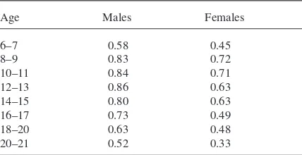
We now examine some relevant descriptive statistics for the sample. Table 2 shows enrollment status of boys and girls by age. As would be expected, Conakry has substantially higher enrollment rates than the national (largely rural) averages noted in the introduction, but a large gender gap remains. Boys’ enrollments are consist-ently higher than girls’ and the gap widens with age, reflecting girls’ earlier withdrawal from school. This is especially apparent after age 15: for example, 73% of boys aged 16–17 are in school compared to only 49% of girls. We should note that the relatively high
Table 2
Current enrollment rates by age and sex in Conakry
Age Males Females
6–7 0.58 0.45
8–9 0.83 0.72
10–11 0.84 0.71
12–13 0.86 0.63
14–15 0.80 0.63
16–17 0.73 0.49
18–20 0.63 0.48
20–21 0.52 0.33
other countries for schooling. At least among older children, therefore, leaving home early is associated primarily with mar-riage (for girls) or work or apprenticeship (for boys) and thus also with leaving school. Thus selection of children out of sam-ple should be negatively correlated with unobserved preferences or propensities for schooling, implyingg2> 0. Sinceb2is also positive, the effect of a variable on schooling will be under-(over-)estimated if that variable increases (decreases) selection into the sample of children staying at home. Parental schooling is likely to increase the desire for child schooling and for this reason will also make it more likely that the child does not leave home early. Thus the positive effect of parental education on schooling for a random sample of children will be under-stated by estimation on the at-home sample when there is selec-tivity. With regard to household income, it is likely thatgkand
enrollment rate for boys in this age group does not mean that most boys (let alone girls) in Conakry progress to upper secondary school: all but 4% of enrolled boys aged 16–17 (and a similar proportion of enrolled girls) are still attending either lower secondary school (grades 7–10) or primary school, a reflection of late starting age or high grade repetition.29
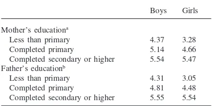
Table 3 shows years of schooling or grade attainment of children 10–18 by sex and education level of the mother and father. We should point out that average schooling levels of parents and especially of mothers is very low: about 75% of the mothers in the sample and 65% of the fathers have less than a primary education, and almost 70% of mothers and 60% of fathers have no schooling at all. In looking at these descriptive results, it should be kept in mind that most of these children (80% of boys and 61% of girls) are currently attending school and thus will likely have an ultimate grade greater
Table 3
Boys and girls aged 10–18: mean years of schooling by sex and level of mother’s and father’s education
Boys Girls Mother’s educationa
Less than primary 4.37 3.28
Completed primary 5.14 4.66
Completed secondary or higher 5.54 5.47 Father’s educationb
Less than primary 4.31 3.05
Completed primary 4.81 4.48
Completed secondary or higher 5.55 5.54 aOn sample with mother schooling data.
bOn sample with father schooling data.
29Enrollments for children who do not live with a parent show a similar pattern of gender differences but are substan-tially lower for both boys and girls. Of course, some older chil-dren in this group have finished their schooling and left home, but younger children not living with a parent (i.e. fostered children) also have lower enrollments. Multivariate analysis on the samples of all boys and all girls under 15 (results available from the authors) indicates an independent negative effect of being fostered on the probability of enrollment controlling for household income and other factors. This does not prove, how-ever, that the practice of fostering is detrimental to child school-ing; in fact, anthropological evidence suggests that fostering is often used by parents to secure an education for their children (see Ainsworth, 1992 and references therein). As noted, living without a parent is correlated with having been born outside of Conakry, which for most such children would mean a rural area where schooling opportunities are relatively limited. Fostered children’s access to schooling in Conakry may thus be superior to what it would have been in the place of origin, even if it is inferior to that of native born children or those living with a parent.
than their current grade. Because of this, the association of parental education and completed schooling will be understated by the cross tabulations in the table, which shows the relation of parents’ education to current grade.30 This is a sample censoring problem and is explicitly addressed in the ordered probit model of grade attainment discussed in the previous section. Even with censoring, the table indicates a substantial positive impact of parental education on children’s schooling, especially for girls. Girls whose mothers have less than a completed primary education have, on average, 3.3 years of school compared with about 4.4 years for boys, but girls with mothers who have a completed sec-ondary education have about 5.5 years of schooling, similar to boys. For father’s education the pattern is simi-lar. These figures thus suggest that improvements in the education of parents are associated with greater increases in the schooling of daughters than of sons, an issue addressed in the estimations discussed below.
5. Empirical results
5.1. Years of schooling
Table 4 reports parameter estimates from ordered pro-bit models of years of schooling for boys and girls aged 10–18. For each case we report results from specifi-cations excluding and including the numbers of children by age and sex in the household. As we noted, household composition is expected to influence the demand for schooling by altering the marginal costs of children’s (especially girls’) time. However, while such variables are often included when analyzing schooling behavior, it is possible that household structure, in particular the number of children, is jointly determined with schooling investments. Such endogeneity is inherent in the quan-tity–quality model, in which parents jointly determine the number of children and their “quality” subject to the income constraint, a vector of prices and other exogen-ous factors. This implies that estimates of the effects of siblings, and potentially other variables, on schooling investments will be biased. Naturally, this is less of an issue where parity can be considered largely exogenous. In our sample, contraceptive use is very low and actual
Table 4
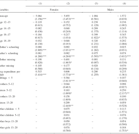
Random effects ordered probit models of years of schooling for males and females aged 10–18 (asymptotict-statistics in parentheses)
(1) (2) (3) (4)
Variables Females Males
Intercept 25.064 25.855 21.004 21.572
(3.156)*** (3.453)*** (0.581) (0.839)
Age 12–13 20.119 20.152 0.238 0.236
(0.613) (0.752) (1.129) (1.092)
Age 14–15 0.082 0.048 0.289 0.245
(0.436) (0.248) (1.375) (1.114)
Age 16–17 20.164 20.217 0.399 0.345
(0.817) (1.034) (1.922)* (1.575)
Age 18–19 0.032 20.048 0.320 0.292
(0.130) (0.193) (1.231) (1.086)
Mother’s schooling 0.088 0.092 0.032 0.025
(3.905)*** (3.931)*** (1.262) (0.931)
Father’s schooling 0.081 0.082 0.075 0.078
(4.260)*** (4.268)*** (3.593)*** (3.632)***
Mother missing 20.198 20.491 0.001 0.131
(0.828) (1.865)* (0.007) (0.536)
Father missing 20.105 20.177 0.028 0.070
(0.588) (0.940) (0.134) (0.299)
Log expenditure per 0.515 0.606 0.200 0.235
adult (3.414)*** (3.774)*** (1.255) (1.361)
Siblings,5 – 20.364 – 20.107
(3.813)*** (0.940)
Brothers 5–12 – 20.044 – 0.096
(0.463) (0.927)
Sisters 5–12 – 0.163 – 0.250
(1.699)* (2.137)**
Brothers 13–20 – 0.158 – 0.100
(1.609) (0.835)
Sisters 13–20 – 0.299 – 20.059
(2.448)** (0.528)
Other children,5 – 0.075 – 20.113
(0.946) (1.571)
Other children 5–12 – 0.031 – 20.076
(0.493) (1.170)
Other boys 13–20 – 0.050 – 0.054
(0.572) (0.590)
Other girls 13–20 – 0.074 – 0.188
(0.760) (1.753)*
Continued.
and desired numbers of children are high.31Still, women or households may indirectly exercise control over fer-tility, for example through the time (of the mother) devoted to schooling, which affects the age of marriage and thus possibly also parity.
31A detailed interview on fertility history, including ques-tions about contraceptive practices, was given to a randomly selected woman from each household as part of the survey. Less than 5% of the women in this subsample who were of childbear-ing age reported uschildbear-ing any form of contraception. The number of children desired, while smaller for women under 35 than
In the absence of any plausible instruments to control for the endogeneity of children, we deal with the poten-tial endogeneity problem simply by estimating the mod-els both with and without the numbers of children (i.e. household members under 21 years old).32The latter will
over 35, was nonetheless between 6.0 and 6.5 for the former. A complete discussion of the results for the fertility survey can be found in Desai, Sahn and del Ninno (1992).
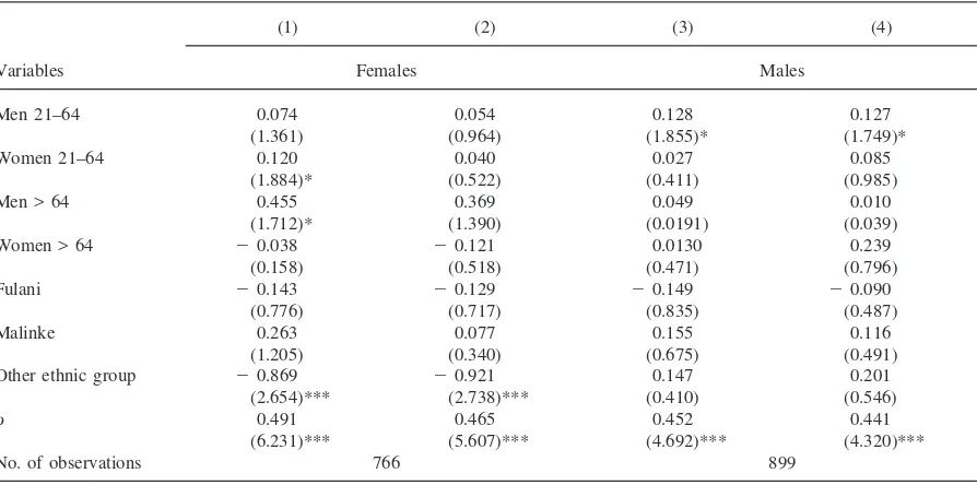
Table 4 Continued.
(1) (2) (3) (4)
Variables Females Males
Men 21–64 0.074 0.054 0.128 0.127
(1.361) (0.964) (1.855)* (1.749)*
Women 21–64 0.120 0.040 0.027 0.085
(1.884)* (0.522) (0.411) (0.985)
Men > 64 0.455 0.369 0.049 0.010
(1.712)* (1.390) (0.0191) (0.039)
Women > 64 20.038 20.121 0.0130 0.239
(0.158) (0.518) (0.471) (0.796)
Fulani 20.143 20.129 20.149 20.090
(0.776) (0.717) (0.835) (0.487)
Malinke 0.263 0.077 0.155 0.116
(1.205) (0.340) (0.675) (0.491)
Other ethnic group 20.869 20.921 0.147 0.201
(2.654)*** (2.738)*** (0.410) (0.546)
r 0.491 0.465 0.452 0.441
(6.231)*** (5.607)*** (4.692)*** (4.320)***
No. of observations 766 899
Notes: Estimates for threshold parameters not shown. * Significant at 10% level; ** significant at 5% level; *** significant at 1% level.
be the appropriate reduced-form schooling demand model as long as the omitted variables are correctly assumed to be endogenous and all relevant exogenous variables are included.33Of course, the relation of family size and structure to children’s schooling is itself of
con-relatives come to live in the household to assist in housework. Estimation of models excluding all household structure covari-ates (for current enrollment and school departures as well as years of schooling) revealed no substantive changes in the esti-mates for parental education while reducing the effects of household per adult expenditures. The latter is not surprising given the correlation of such a measure of household income with household size and structure. However, the pattern by gen-der in the estimates for expenditures and their significance lev-els (discussed below) did not change.
33These conditions for obtaining the correct reduced form need to be emphasized. If the household or fertility variables in fact are exogenous determinants of schooling, their exclusion implies a misspecified reduced form, which will suffer from omitted variable bias if the included covariates are correlated with the excluded fertility variables. If fertility is correctly assumed to be endogenous to schooling decisions, these vari-ables do not belong in a reduced form, but strictly speaking, one should include all exogenous determinants of fertility and typically only some of these (e.g. a woman’s education) are observed. If unobserved exogenous determinants of the price of child quantity are correlated with the included exogenous variables, the estimates on the latter will suffer from omitted variable bias (Browning, 1992). There is probably little vari-ation in omitted determinants of fertility within Conakry, which would suggest that there is no such bias, but this may not be the case throughout Guinea. Mothers of children in the sample
siderable interest. For the results of the models including these variables, it may be possible at least to assess the direction of the simultaneity biases that might occur, as we discuss below.
We first consider the estimates in Table 4 for parental education and log expenditures per adult, which is included as a measure of household permanent income. More years of schooling of both mothers and fathers lead to higher grade attainment of girls (columns 1 and 2); the estimates are similar for the models with and without child variables. Better schooling of fathers also raises the grade attainment of boys (columns 3 and 4), but school-ing of mothers does not: the mother’s coefficients in the boys’ ordered probits are only about a third as large as those for father’s schooling and do not approach statisti-cal significance in either specification. Similarly, house-hold permanent income, proxied by the log of per adult expenditures, has a positive and highly significant effect on grade attainment of girls in both models, but does not affect boys’ schooling.34 The coefficients on
expendi-who migrated to Conakry from different regions of the country after the start of their childbearing years may indeed have been exposed to differing unobserved determinants of fertility that are correlated with the included regressors.
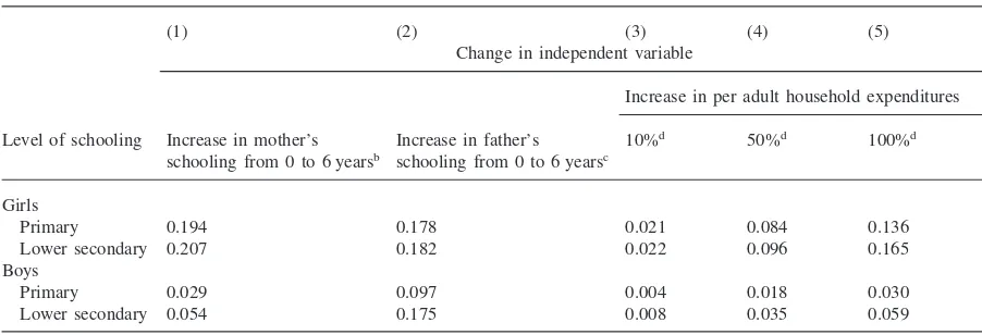
Table 5
Effects of changes in parental education and household per adult expenditures on predicted probabilities of primary and lower second-ary schooling of girls and boysa
(1) (2) (3) (4) (5)
Change in independent variable
Increase in per adult household expenditures Level of schooling Increase in mother’s Increase in father’s 10%d 50%d 100%d
schooling from 0 to 6 yearsb schooling from 0 to 6 yearsc Girls
Primary 0.194 0.178 0.021 0.084 0.136
Lower secondary 0.207 0.182 0.022 0.096 0.165
Boys
Primary 0.029 0.097 0.004 0.018 0.030
Lower secondary 0.054 0.175 0.008 0.035 0.059
aCalculated from ordered probit model results in Table 4 (see text).
bShows the change in the probability of completing the indicated schooling level resulting from an increase in mother’s schooling from 0 to 6 years.
cShows the change in the probability of completing the indicated schooling level resulting from an increase in father’s schooling from 0 to 6 years.
dShows the change in the probability of completing the indicated schooling level resulting from an increase in household expenditures by the indicated amount.
tures for both girls and boys are somewhat larger (by about 15%) when the full set of household covariates is included, but in either specification the pattern by gender is the same. These estimates thus suggest important dif-ferences by gender in parental education and expenditure effects. However, the ordered probit coefficients do not measure the actual impacts of these and other covariates on years of school, reflecting the non-linear structure of the model. Instead, the actual impacts can be assessed through comparative statics calculations based on the estimates and the data. Table 5 presents the results of such an exercise.
The table shows, first, the effects of mother’s and father’s primary education on the probabilities of daught-ers and sons completing primary school (i.e. on prob [years of schooling $ 6]) and lower secondary school
respect to preferences such that those with a propensity to invest more in their children’s education work more and earn more income, implying an upward bias to the estimated effects of expenditure or income. Experiments with predicted expendi-tures, using as instruments household assets and non-labor income, in general yielded very poor results: the coefficients on expenditures were not at all robust to changes in the specifi-cations of the predicting and schooling equations and were occasionally wrongly (negatively) and even significantly wrongly, signed. Thus we rely on reported values of household expenditures in spite of the potential for endogeneity.
(prob [years of schooling$ 10]).35The change in the probability is calculated as the difference in the prob-abilities of completing a given level when the parent has 6 years of schooling and when he or she has zero years of schooling, evaluating all other variables at the sample means for girls or boys. Since average levels of school-ing of parents in the sample are low, the no-schoolschool-ing to primary focus is appropriate. Also shown are the effects on primary and lower secondary completion of increases in per adult expenditures of 10, 50 and 100% above mean expenditures. We use the estimates from the models including the full set of household composition variables (columns 2 and 4 in Table 4) to calculate the comparative statics, but the results for both parental edu-cation and income were robust to changing the basis of the calculations from the full to the reduced (excluding children covariates) model estimates.
As shown in the first column, mother’s primary schooling raises the probability that a girl will achieve at least a primary education by about 20 percentage points over the no maternal schooling base case, with a similar impact on lower secondary schooling. Note that these are absolute changes in the predicted probabilities (e.g. in the case of primary completion, from 0.58 when the mother has no education to 0.77 when the mother
has a primary education).36 These effects on girls are much larger than the calculated maternal schooling impact on sons’ primary and secondary attainment prob-abilities (just 0.03 and 0.05 percentage points, respect-ively; recall as well that the parameter estimates in the boys’ ordered probit model were not significant).
Column 2 of Table 5 shows the effects of father’s schooling. For primary school completion, paternal schooling impacts, like maternal schooling effects, are higher for daughters than sons, though the difference in the daughter and son effects is much less dramatic than for maternal schooling. For lower secondary completion paternal schooling effects are similar for daughters and sons. Comparing maternal and paternal impacts (reading across columns 1 and 2), in the case of girls, the effects of father’s primary education on primary and lower sec-ondary completion are similar to the effects of mother’s education, but for boys father’s primary education has impacts on primary and secondary completion that are more than three times greater than those of mother’s pri-mary education.
What stands out most strongly from these simulations is that improvements in maternal schooling have much greater impacts on the education of daughters than of sons. Paternal schooling overall also seems to favor daughters’ education over sons’, but to a lesser degree. Thus the relative benefit to girls, defined as the differ-ence in the improvements in girls’ and boys’ schooling, is greater from mother’s education than from father’s education. One explanation for this, noted above, is rooted in a bargaining model of resource allocation within the household: educated mothers have strong pref-erences for educated daughters, and being educated con-fers the power to direct household resources toward daughters’ human capital development. Also as noted, however, the findings are consistent with unified house-hold preferences under interhousehouse-hold heterogeneity in preferences for schooling daughters.37 The data do not allow us to distinguish these explanations empirically,
36Thepercentage, i.e. proportional, increase in probability in the case of primary completion is 0.32 (50.19/0.58).
37It is also possible that a stronger maternal education effect on daughters arises because mothers spend more time with daughters, so improvements in mother’s schooling will raise the efficiency of learning (and demand for schooling) of girls more than boys, with the opposite being the case for fathers and sons; this possibility is pointed out by Thomas (1992) in the context of child health. This is consistent with common parental prefer-ences, but only if differing mother and father time allocations are determined exogenously by cultural factors or technological (efficiency) considerations rather than preferences of mothers to be with daughters and fathers to be with sons.
but the first interpretation is consistent with what is known about households in West Africa.38
Comparison of the first two columns of Table 5 with the last three columns indicates that parental primary education has impacts on children’s schooling, and especially daughter’s schooling, that are equivalent to very significant increases in household income, proxied by per adult expenditures. Both mother’s and father’s primary schooling have substantially larger impacts on girls’ primary and secondary completion probabilities than a doubling of household income.39 Some caution is necessary in making these comparisons since we are inferring the effects of large changes in parental edu-cation and income from estimates that relate to marginal changes in the independent variables. Consistent with the parameter estimates discussed above, additions to house-hold expenditures have much larger calculated effects on girls than boys for each level of schooling attainment. These differences are consistent with studies of other developing countries. DeTray (1988) and Gertler and Glewwe (1992) report higher income elasticities for girls’ schooling in Malaysia and Peru, respectively, while Schultz (1985) finds a similar pattern using cross-national data.40
We next examine the effects of household structure on years of schooling. The extended ordered probit
mod-38The linear schooling specification used in the models is potentially restrictive, so we also experimented with quadratics in years of mother and father schooling as well as with dummy variables for parental schooling levels. These experiments con-firmed the basic findings. In particular, in specifications using dummy variables for lower primary, upper primary, and second-ary schooling of the parents, maternal schooling impacts for all levels were significant for girls’ grade attainment but none were significant for boys’. Father’s primary and schooling dummies, in contrast, were significant for both boys and girls. Similar experiments with the current enrollment probits specifications reviewed in the next section yielded the same conclusion.
39The effect of mother’s schooling may, in fact, be underesti-mated. The simulations do not account for changes in other factors that may be induced by changes in maternal education. In particular, more educated women tend to have fewer chil-dren, which may permit higher investments in schooling for each.