Vol. 42 (2000) 483–521
Mixed strategies and iterative elimination of strongly
dominated strategies: an experimental investigation of
states of knowledge
Amnon Rapoport
a,∗,1, Wilfred Amaldoss
b,2aDepartment of Mangement & Policy, The Eller School of Business and Public Administration,
405 McClelland Hall, University of Arizona, Tucson, AZ 85721, USA
bKrannert Gradaute School of Management, Purdue University, West Lafayette, IN 47906, USA
Received 5 May 1998; received in revised form 30 August 1999; accepted 31 August 1999
Abstract
The iterative elimination of strongly dominated strategies (IESDS) and mixed-equilibrium solu-tion concepts are studied in an iterated two-person investment game with discrete strategy spaces, non-recoverable investments, and either equal or unequal investment capital. In this game, the player investing the largest amount wins the competition and receives a fixed reward; ties are counted as losses. Both cases of symmetric and asymmetric dyads are studied theoretically and experimen-tally. Results from two experiments provide support for the mixed-strategy equilibrium solution on the aggregate but not the individual level, and evidence for a hierarchy of bounded IESDS. © 2000 Elsevier Science B.V. All rights reserved.
JEL classification: C72; C92
Keywords: Mixed strategies; Iterative deletion of strongly dominated strategies; Bounded rationality; Adaptive learning
1. Introduction
Iterative elimination of strongly dominated strategies (IESDS) and mixed-strategy Nash equilibrium are two of the most basic solution concepts of non-cooperative game theory. The assumptions on the players’ state of knowledge that are sufficient to derive these
∗Corresponding author. Tel.:+1-520-621-9325; fax:+1-520-621-4171.
E-mail address: [email protected] (A. Rapoport) 1Professor of Management and Policy.
2Assistant Professor of Marketing.
solution concepts are by now well known. To state them, consider a finite non-cooperative game in strategic (normal) form, which consists of a finite set of players, a finite set of choices (strategies) for each player, and a payoff function assigning a payoff for each player for every specification of choices by all the players. Call a fact mutual knowledge if every player knows it, and common knowledge if everyone knows it, everyone knows that everyone knows it, and so on ad infinitum. Define the conjecture of a player as that player’s probability assessment over the strategy choices of the other players. The following propositions have been proved with differing degrees of formality (see Brandenburger (1992), and references cited therein):
1. Suppose that the structure of the game and rationality of the players are common knowl-edge. Then, each player chooses an iteratively undominated strategy.
2. Suppose that there are only two players, and that the structure of the game, rationality of the players, and their conjectures are mutual knowledge. Then, the players’ conjectures constitute a mixed-strategy Nash equilibrium.
3. For more than two players, suppose that there is a common prior on the set of states of the world, that at some state, the structure of the game and rationality of the players are mutual knowledge, and that the conjectures of the players are common knowledge. Then, for each player, all the other players hold the same conjectures about that player, and the resulting profile of conjectures constitutes a mixed-strategy Nash equilibrium. Several brief comments on these propositions are in order. IESDS — a relatively weak solution concept — is based on the assumption of common knowledge of rationality. In certain games such as the finitely iterated Prisoner’s Dilemma and Centipede games, IESDS leads to counter-intuitive results. As noted by Aumann (1996) (pp. 130–131), “common knowledge of rationality is a very strong assumption, much stronger than simple rationality, and in some situations may just be too much to ask for.” Common knowledge of rationality is required in order to state a sufficient condition applying to all finite games. However, for finite games that are typically played in the laboratory, there is an obvious bound — which in many cases is quite small — on the levels of knowledge, or depth of reasoning, needed to conclude that players actually choose iteratively undominated strategies. With regard to the mixed-strategy Nash equilibrium, it turns out that the assumptions on the players’ state of knowledge that lead to their conjectures being in equilibrium depend significantly on the number of players. In particular, when there are only two players, mutual knowledge of the conjectures is sufficient, but when there are more than two players, the stronger requirement of common knowledge of conjectures is required.
1.1. Previous studies
of these experiments are that (1) when the strategy space of each player includes only very few elements, the aggregate results are described quite well by the mixed-strategy Nash equilibrium; (2) the descriptive power of this solution concept decreases as the number of elements in the strategy set increases; and (3) the mixed-strategy equilibrium cannot account for the persistent and systematic sequential dependencies found on the individual level. The evidence seems to suggest that people do not start their play by randomizing over their pure strategies. Rather, they gradually reach equilibrium play through some process of adaptation (Binmore et al., 1996). The experimental evidence seems to be more consistent with reinforcement-based learning than belief-based models (Mookherjee and Sopher, 1997).
Experimental studies of IESDS have mostly focused on the degree or depth of iterated dominance. As such, they have contributed to the understanding of the limitations on the human cognitive system. In addition to the multitude of studies of the two-person finitely iterated Prisoner’s Dilemma game, McKelvey and Palfrey (1992) studied the two-person Centipede game, and Stahl and Wilson (1995) examined a class of 3×3 games. The most prominent paradigm has been the Beauty Contest game, numerous variations of which have been recently investigated by Nagel (1995, 1999), Camerer and Ho (1996), Stahl (1996), Duffy and Nagel (1997), and Ho et al. (1998). In its simplest form, the basic game proceeds as follows. Each of n players chooses simultaneously and privately a number xi, xi =1,2, . . . , n, from a fixed and commonly known real-valued interval, say [0, 100]. The
winner is the player whose chosen number is closest top(x1+x2+ · · · +xn)/n, where p<1 is a predetermined and commonly known constant. The winner is awarded a fixed prize; in the case of a tie, the prize is split equally among the tied players. The game is repeated several times with no rematching of players. Iterated elimination of weakly (rather than strongly) dominated strategies leads to a unique solution where, in our example, each player chooses zero. The general finding of the different variants of the Beauty Contest game is that most subjects of groups ranging in size between 4 and 17 do not engage in a high number of iteration steps. “The level of reasoning does usually not go beyond level 3 as observed in many other studies” (Nagel, 1999). However, the depth of reasoning and rate of learning seem to depend on group size, sophistication of the players, and previous experience with the game.
The present paper examines yet another game, called the Investment game, which allows for the simultaneous investigation of the IESDS and mixed-strategy equilibrium solution concepts. As this game was inspired (Rapoport and Amaldoss, 1996) by our study of com-petition between two firms for the development of a new technology product, and as the instructions for the two experiments were presented in these terms, we motivate the game within this context. No claim is made here that this game — an abstraction — can serve as a complete model of such R&D competitions.
The paper is organized as follows. In Section 2, we first consider the case of symmetric players (firms) with equal endowments (R&D budgets), formulate it as a non-cooperative two-person game in strategic form, and then construct the symmetric Nash equilibrium solution for the game. In equilibrium, each player k (k=i, j) randomizes over the entire set
distributions, one for the ‘strong’ player and the other for the ‘weak’ player. We end this section with a comparison of the Investment game with previous games proposed to assess the descriptive power of the IESDS and mixed-strategy equilibrium solution concepts. Section 3 describes an experiment designed to study the symmetric case of the investment game, and Section 4 the asymmetric case. Section 5 attempts to account for the major patterns observed in the results of both experiments by adaptive learning. Section 6 concludes the paper.
2. Problem statement and equilibrium solution
We consider the case of two firms competing in the development of a new technology product. The successful firm obtains patent and monopoly rights to the product, whereas the losing firm gets nothing. Like O’Neill (1986), we assume a discrete model and com-monly known budgetary constraints. We further assume that whoever invests more wins the competition, because the amount spent on R&D could potentially influence the successful development and patenting of the product (e.g., Besanko et al., 1996).
Formally, we consider two players (firms), i and j, with endowments (R&D budgets) ei
and ej, respectively, assumed to be commonly known. Each player k (k=i, j) invests the
amount ck (ck =0,1, . . . , ek). Investments are assumed to be made simultaneously; they
are not recoverable. Let r denote the payoff associated with winning the competition; we assume that the value of r does not depend on the actual investments ci and cj, and that r>ek>1. Let s denote the amount that each player receives in the event that both players
make the same investment (ci=cj). The resulting payoff structure has the following form:
Ui(ci, cj)=
The most common assumption in patent race models is that s=r/2; if the two firms
in-vest the same amount in the development of the new product (ci=cj), then the reward r
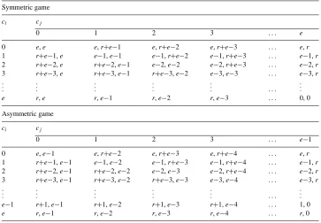
Table 1
Payoff matrices for the symmetric and asymmetric Investment gamea Symmetric game
power capability, biological and chemical weapons) results in a stalemate (and conse-quently, total loss of the resources expended in developing the technology). The sec-ond reason for this assumption is that it drives the theoretical results presented below, which imply randomization over all the strategies when the players are symmetric (ei=ej), and IESDS followed by randomization over the iteratively undominated
strate-gies when the players are not symmetric (ei6=ej). We wish to study these non-obvious
strategic implications in the context of a competition for the development of a new product.3
2.1. Symmetric players
The competition between the two players is modeled as a non-cooperative two-person game in strategic form with complete information and discrete strategy spaces
ci = {0,1, . . . , ei}andcj = {0,1, . . . , ej}. Consider first the case of symmetric
play-ers, namely, ei=ej. To simplify notation, define e≡ei=ej. The upper panel of Table 1
presents the payoff matrix for the general case of the Investment game.
Inspection of Table 1 verifies that neither player has dominated strategies and that the game has no equilibrium solution in pure strategies. The following proposition is proved in Appendix A.
Proposition 1. If the two players are symmetric and risk-neutral, there exists a unique
mixed-strategy Nash equilibrium given by
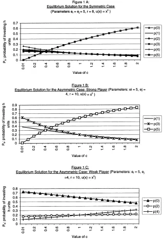
For example, if e=5 and r=8, as in Experiment 1 below, then in equilibrium, each player invests 0, 1, 2, 3, or 4 units with probability 1/8, and 5 units with probability 3/8. The probability of a tie in this case is 7/32, and the expected payoff for each player is 5 units.
There are three important features of the equilibrium solution, all experimentally testable, which warrant discussion. First, Proposition 1 implies that the expected payoff of each player is independent of the reward r. In equilibrium, substantially increasing the reward for winning the competition affects the mixed strategy ppp, but not the expected payoff. Therefore, symmetric players adhering to the equilibrium solution should be indifferent to the magnitude of the reward associated with winning the competition when playing the Investment game.
Second, by setting ck=0, each player can guarantee the value of his or her budget; ck=0 implies that Uk(0, 0)=ek. The equilibrium strategies do not yield a higher payoff
than e; indeed, they do not even guarantee this payoff. As noted by Aumann and Maschler (1972), who observed the same phenomenon in a class of two-person zerosum games, if the equilibrium strategies are to be played at all, they are presumably played with the hope that each player will obtain his or her equilibrium payoff. But then, why play ‘with hope’ when the two players could each guarantee the same payoff by choosing minimax rather than equilibrium strategies? Therefore, it is doubtful whether players will invest any amount in the Investment game. Randomization in the Investment game seems to be less likely to occur than in the various two-person zerosum games studied experimentally by O’Neill (1987), Rapoport and Boebel (1992), and Mookherjee and Sopher (1994, 1997).
Thirdly, the equilibrium outcome is Pareto-deficient. If the game is iterated in time and the two players tacitly coordinate their actions by jointly alternating between 0 and 1, then the expected payoff for each player is (r+2e−1)/2. Unlike the equilibrium expected payoff, this expected payoff increases linearly in r. For the parameters used in Experiment 1, the difference between the two expected payoffs is substantial. (For example, if e=5 and r=20, then the expected payoff almost triples from 5 to 14.5). Moreover, expected payoffs exceeding the equilibrium payoffs can be obtained even without tacit coordination (e.g., by each player k independently randomizing between ck=0 and ck=1 with equal
The equilibrium solution can be constructed for the more general case that does not require risk-neutrality. Denote the utility of x by u(x) and assume that u(x) is increasing. If the two players are symmetric and share the same attitude to risk, then there exists a unique mixed-strategy Nash equilibrium (see Rapoport and Amaldoss, 1996) given by
ppp=(p0, p1, . . . , pe)where the probability ph(h=0,1, . . . , e−1) is computed from ph=
u(e)−u(e−h−1)
u(r+e−h−1)−u(e−h−1)−
u(e)−u(e−h)
u(r+e−h)−u(e−h) (2)
and
pe=
u(r)−u(e) u(r) .
In equilibrium, each player’s expected payoff is u(e).
It is easy to verify that, if u(x)=x, the solution in Eq. (2) reduces to the one in Eq. (1). It
is also easy to verify that if the (common) utility function u(x) is concave, the probability of investing the entire capital, pe, decreases.4 To illustrate this case, assume that u(x)=xc
(0<c), e=5, and r=8. Setting c=0.7, Eq. (2) yields
ppp=(p0, p1, p2, p3, p4, p5)=(0.1461,0.1438,0.1414,0.1392,0.1492,0.2804).
Changing the reward from r=8 to r=20, while keeping e=5 and c=0.7 as before, we obtain
ppp=(p0, p1, p2, p3, p4, p5)=(0.0675,0.0685,0.0704,0.0745,0.0981,0.6211).
Fig. 1 displays the mixed-strategy equilibrium solution for a power utility function where
e=5 and r=8. The probabilities are portrayed as a function of risk aversion, measured here by the power parameter c (0<c61). As the degree of risk aversion increases (c decreases from 1 to 0), the probability of investing ck=e decreases from 0.375 to 0, while the other
five choice probabilities increase but at slightly different rates.
2.2. Asymmetric players
The formulation of the asymmetric case is the same as above with the only exception that ei6=ej. Without loss of generality, assume that ei>ej, and refer to players i and j as the strong and weak players, respectively. As in the case of symmetric players, we assume that r>ei>ej>1.
When the players are asymmetric, it is sufficient to consider the case ei=ej+1. This
is so because, if ei>ej+1, any strategy of player i dictating ci=ej+s (s>1) is strongly
dominated by the strategy ci=ej+1. To simplify notation, we denote player i’s endowment
by e and player j’s endowment by e−1, and designate the strategies of players i and j as rows and columns, respectively. The lower panel of Table 2 presents the payoff matrix for the asymmetric Investment game.
When the players are asymmetric, their strategic considerations differ from the ones in the symmetric Investment game. The strong player can guarantee himself a payoff of r by
Table 2
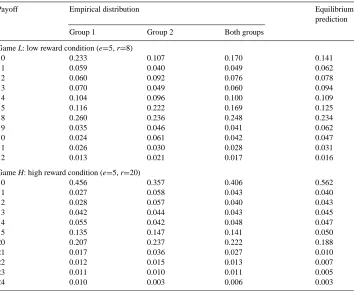
Aggregate distribution of payoffs in the symmetric casea
Payoff Empirical distribution Equilibrium
aThe relative frequencies were computed using the payoffs obtained over 80 trials. Group 1 played Game L in the first 80 trials and Game H in the last 80 trials. Group 2 played Game H in the first 80 trials and Game L in the last 80 trials. Each group includes 18 subjects.
investing his entire budget, e. Anticipating that, the weak player can then invest cj=0 (and
receive a net payoff of e−1). If, however, player i anticipates that player j will invest nothing, he is better off investing 1 (rather than e). But once the strong player does not invest his entire budget, he is no longer sure of winning.
Denote the strategy spaces of players i and j by ci={0,1, . . . , e}and cj={0,1, . . . , e−
1}, respectively, and assume that both players are risk-neutral. Then, the equilibrium strate-gies of the two players are characterized as follows (see proof in Appendix A):
Proposition 2. Pure strategies are iteratively eliminated in the order: row 0, column 1, row
2, column 3,. . ., rowe−1 (if e is odd) or columne−1 (if e is even).
and the weak player randomizes over her even-numbered strategies (including strategy 0j)
If e is odd, the strong player randomizes over his odd-numbered strategies according to the probability vector
and the weak player randomizes over her even-numbered strategies according to the prob-ability vector
In equilibrium, the expected payoff of the strong player is eitherr+1, if e is even, or r, if
e is odd. The expected payoff of the weak player for both odd and even values of e equals e−1.
The equilibrium solution for the asymmetric case shares some of the features of the solution for the symmetric case. However, when the players are asymmetric, the expected payoff of the strong player depends on the value of r, while the weak player’s expected value does not. Therefore, if they adhere to equilibrium play, the strong player should prefer the reward to be higher, whereas the weak player should be indifferent to the size of the reward.
As in the symmetric case, the weak player can guarantee her budget, e−1, by investing 0. Similarly, the strong player can guarantee the reward r by investing e. When e is odd, as in our Experiment 2, the expected values of the two players under equilibrium play are e−1 and r. However, unlike minimax play, the equilibrium solution does not guarantee these values to the weak and strong players. Therefore, exactly as in the symmetric case, we have no reason to expect the weak player to invest any positive amount or the strong player to invest any amount smaller than e.
Another experimentally testable implication is that the probability vectors of the strong and weak players, in each case defined over the strategies that survive IESDS, are symmetric: compare Eq. (3) with Eq. (4) and Eq. (5) with Eq. (6).
A third testable implication is that both players only play strategies that survive IESDS. Eqs. (3)–(6) imply that about half of the pure strategies of each player survive IESDS. If
e is relatively large, it is highly unlikely that, without knowledge of non-cooperative game
Proposition 2 also assumes risk neutrality. Construction of the mixed-strategy equilibrium solution for the more general case, where the players can share other attitudes toward risk, requires the simultaneous solution of linear equations whose number increases in e. Therefore, we provide below only the equilibrium solution for the investment capital used in Experiment 2, namely, e=5.
If the strong and weak players are endowed with investment capital of 5 and 4, respec-tively, then after the iterative deletion of row 0, column 1, row 2, column 3, and row 4, the strong player should randomize over his iteratively undominated strategies 1, 3, and 5 with respective probabilities
p1=
u(4)−u(2)
u(r+2)−u(2), (7)
p3=u(4)[u(r+2)−u(r)]−u(r)[u(4)−u(2)]
u(r)[u(r+2)−u(2)] , (8)
and
p5=
u(r)−u(4)
u(r) . (9)
After iteratively deleting her dominated strategies, the weak player should randomize over her undominated strategies 0, 2, and 4 with respective probabilities
p0=
u(r)−u(4)
u(r+4)−u(4), (10)
p2=
u(r)
u(r+2)−u(2)+
u(4)u(r+2)−u(2)u(r+4)
[u(r+4)−u(4)][u(r+2)−u(2)]
− u(r)
u(r+4)−u(4), (11)
and
p4= u(r+2)−u(r)
u(r+2)−u(2). (12)
The expected payoffs for the strong and weak players are u(r) and u(e−1), respectively. It is again possible to verify that in the case of risk neutrality, Eqs. (7)–(9) reduce to Eq. (5) and Eqs. (10)–(12) reduce to Eq. (6). With risk aversion, the probability that the strong player invests his entire capital (Eq. (9)) or the weak player invests zero capital (Eq. (1)) decreases.
Contest game has a unique pure-strategy equilibrium at zero, whereas the equilibrium for the Investment game is in mixed strategies. Fourth, the Beauty Contest game is solved by iterative elimination of weakly rather than strongly dominated strategies. As such, it actually tests a slightly different mental process because the set of strategies that survive iterated elimination of weakly dominated strategies may depend on the order in which strategies are being eliminated (Osborne and Rubinstein, 1994). The fifth and possibly most important difference between these two games is that, when the number of players is restricted to two, as in the Investment but not the Beauty Contest game, a weaker hypothesis about the players’ state of knowledge can be tested. As a result, one may expect deeper levels of reasoning than those typically observed in the Beauty Contest game.
3. Experiment 1: the Investment game with symmetric players
3.1. Subjects
Thirty-six undergraduate and graduate students from the University of Arizona partici-pated in the study. Subjects were recruited through advertisements placed on bulletin boards on campus and class announcements. They were promised monetary reward contingent on performance for participation in a decision making experiment. Subjects were run in groups; 18 subjects participated in Group 1 and another 18 in Group 2.
3.2. Procedure
Each experiment consisted of a single session lasting about 2 h. Upon arrival at the laboratory, all the group members were randomly seated in separate booths. Subjects read the instructions for the experiment5 on their individual computer terminals. Any form of communication before or during the experiment was not possible.
Subjects were randomly matched into pairs on each trial. In particular, on each trial, the 18 group members were rematched to form nine pairs according to a predetermined assignment schedule. Subjects had no way of knowing the identity of their competitors on any given trial. The assignment schedule ensured that each subject would be matched with each of the other group members approximately the same number of times, and that a subject would not be paired with the same competitor twice in a row.
The instructions explained and demonstrated the Investment game. The game was not presented in matrix form. Rather, at the beginning of each trial, the subjects were only informed of the values of ei, ej, r, and rules of the game. Once the subjects made their
investments privately, the computer compared each player’s investment with that of the other dyad member and determined the winner. Ties were counted as losses. At the end of each trial, each player k was informed of (1) the values of ci and cj, (2) the winning player
(i or j), and (3) his or her reward for the trial (Uk).
Each group participated in two experimental conditions (or games) in a within-subjects design. The payoff parameters for these two games were
Low Reward Condition (Game L): ei=ej=5, r=8.
High Reward Condition (Game H): ei=ej=5, r=20.
Each stage game was played repeatedly (with the same value of r) for 80 successive trials. The subjects in Group 1 were presented first with Game L (Phase 1: trials 1–80) and then with Game H (Phase 2: trials 81–160), for a total of 160 trials. The order of presentation of the two games was reversed in Group 2.
Investments were made in terms of a fictitious currency called ‘franc’. At the end of the experiment, the individual payoffs were totaled and converted into US dollars at the exchange rate of 80 francs=US$ 1.00. In addition, subjects were paid a US$ 5.00 show-up fee.6
4. Results
We first examine the distribution of payoffs received by subjects and assess whether the payoffs are insensitive to the size of reward as predicted by theory. Then, we study the strategy profiles played by subjects both at the aggregate and individual levels. Finally, we investigate how subjects came to conform to the theoretical predictions.
4.1. Payoffs
Table 2 presents the relative frequency distributions of payoffs for Game L (upper panel) and Game H (lower panel). The realizable payoffs for Game L (column 1 of the up-per panel) are 0,1, . . . ,5,8,9, . . . ,12, whereas the ones for Game H (lower panel) are 0,1, . . . ,5,20,21, . . . ,24. Columns 2, 3, and 4 of each panel present the observed rel-ative frequencies of payoff for Group 1, Group 2, and across both groups, respectively. The right-hand column of each panel shows the probability distribution of payoff under equilibrium play.
4.2. Game L
The expected payoff per trial under equilibrium play is e=5. The mean payoff of both groups in Game L is equal to 5.536. This mean does not differ significantly from the theoretical value (z=0.335, p>0.36). Similar results hold when the relative frequencies of each group are examined separately. The mean payoff earned by Group 1 is 4.456 (z=1.378,
p>0.08) and by Group 2 is 5.362 (z=0.986, p>0.16). Under equilibrium play, the variance of the payoffs in Game L should equal 11.875. In actuality, the variance of the observed payoffs computed across the subjects in both groups is 11.825; this variance does not differ
significantly from the theoretical value (χ2=158.3, p>0.1). Similar results obtain on the group level: the variance of payoffs is 12.460 in Group 1 (χ2=82.894, p>0.1) and 10.785 in Group 2 (χ2=71.75, p>0.1).
The results are similar when we examine the aggregate distributions of payoffs rather than their mean and variance. The relative frequency distribution of payoffs computed across the subjects of both groups in Game L does not differ significantly from the predicted probability distribution under equilibrium play (Kolmogorov–Smirnov statistic D160=0.03, p>0.2).
Similar results hold for Group 1 (D80=0.093, p>0.2) and Group 2 (D80=0.002, p>0.2).
4.3. Game H
Although the reward r is higher in Game H than Game L by a factor of 2.5, the expected payoff under equilibrium play is the same. The mean payoff per trial computed across the two groups is significantly higher than predicted (combined mean is equal to 6.845,
z=2.705, p<0.004). This result is mainly attributed to Group 2. We cannot reject the null hypothesis in Group 1 (mean=6.357, z=1.43, p>0.076), but have to reject it in the case of Group 2 (mean=7.344, z=2.39, p<0.01). As for the variability of the payoffs in Game H, the theoretical variance under equilibrium play is 64.75. The observed variance computed across both groups (74.45) does not differ from the theoretical value (χ2=182.8, p>0.1). Similar results hold for each of the two groups.
As may be expected from these results, the observed aggregate frequency distribution of payoff computed across both groups differs from the theoretical distribution under equilib-rium play (D160=0.159, p<0.01). The null hypothesis is rejected in the case of Group 2
(D80=0.206, p<0.01) but not Group 1 (D80=0.137, p>0.05).
A strong testable implication of the equilibrium solution is that the mean payoff per trial in the symmetric case of the Investment game is independent of the reward r for winning the competition. This implication is clearly rejected when we compare to each other the mean payoffs in Games L and H (z=2.64, p<0.04). The observed payoffs in the symmetric Investment game seem to be sensitive to the reward condition.
4.4. Strategy profiles
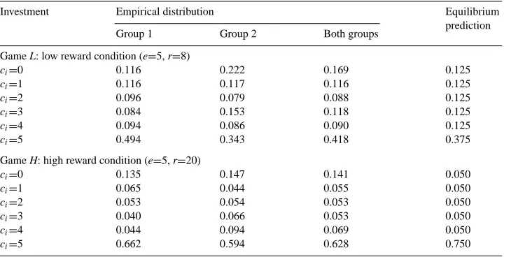
Table 3 shows the observed relative frequencies of choice of the six investment strategies. Computed across subjects and trials, the frequencies are presented separately in terms of group and game. The most notable finding is that in both Games L and H the subjects did not choose to always play the minimax strategy of zero investment. Rather, most of the subjects played all six pure strategies. As predicted, strategy ck=e was chosen considerably more
often than any other strategy. Also, as predicted, the subjects chose to invest their entire budget significantly more often when the reward for winning the competition was increased from 8 to 20. The Kolmogorov–Smirnov test of goodness of fit indicates no significant difference between the observed and theoretical frequency distribution of choices under equilibrium play in Game L (D80=0.119, p>0.2, for Group 1; D80=0.097, p>0.2, for Group
2; and D160=0.44, p>0.2, for the combined groups). A marginally significant difference
Table 3
Aggregate distribution of investment in the symmetric case
Investment Empirical distribution Equilibrium
prediction
Group 1 Group 2 Both groups
Game L: low reward condition (e=5, r=8)
ci=0 0.116 0.222 0.169 0.125
ci=1 0.116 0.117 0.116 0.125
ci=2 0.096 0.079 0.088 0.125
ci=3 0.084 0.153 0.118 0.125
ci=4 0.094 0.086 0.090 0.125
ci=5 0.494 0.343 0.418 0.375
Game H: high reward condition (e=5, r=20)
ci=0 0.135 0.147 0.141 0.050
ci=1 0.065 0.044 0.055 0.050
ci=2 0.053 0.054 0.053 0.050
ci=3 0.040 0.066 0.053 0.050
ci=4 0.044 0.094 0.069 0.050
ci=5 0.662 0.594 0.628 0.750
p<0.05). On further analysis, we find that the investment frequencies conform to the equi-librium prediction in Group 1 (D80=0.103, p>0.2) but not in Group 2 (D80=0.156, p<0.05).
These results provide strong support to the equilibrium solution. Given the marginal discrepancy in the observed frequency distribution of choices in the high reward condition, we probed further to understand the reason for it. We find that the mean investment by Group 2 does not differ significantly from the theoretical value (z=1.762, p>0.04). However, the observed variance of choices is considerably different from the theoretical prediction (χ2=189.08, p<0.005). Inspection of the results of Game H shows that strategy ck=0 was
chosen more often than predicted. Such an investment pattern could be a consequence of either a few subjects deviating from equilibrium behavior and playing the minimax strategy of zero investment in most of the trials, or most subjects mixing strategies but investing zero more often than predicted by theory. We will examine this issue further when discussing individual level differences in investment strategy profiles.
4.5. Trends in investment
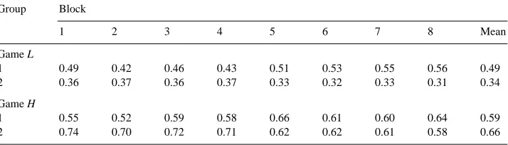
Table 4
Experiment 1: mean proportion of trials on which the entire endowment was invested by game, group, and blocka Group Block
1 2 3 4 5 6 7 8 Mean
Game L
1 0.49 0.42 0.46 0.43 0.51 0.53 0.55 0.56 0.49
2 0.36 0.37 0.36 0.37 0.33 0.32 0.33 0.31 0.34
Game H
1 0.55 0.52 0.59 0.58 0.66 0.61 0.60 0.64 0.59
2 0.74 0.70 0.72 0.71 0.62 0.62 0.61 0.58 0.66
aThere are 18 subjects in each group and 10 trials in each block.
steadily moving towards the equilibrium prediction for Game H. In contrast to Group 1, the corresponding proportions for the subjects of Groups 2 move away from equilibrium play.7
4.6. Individual differences
As the results reported in Tables 3 and 4 pertain to aggregate data, they may conceal considerable individual differences in investment strategy profiles. We suggested earlier that these results are compatible with the hypothesis that there are two distinct segments of subjects: one mixing their strategies, and the other playing the minimax strategy of zero investment.
4.7. Game L
The upper panel of Fig. 2 exhibits the frequency distributions of the number of times the entire budget was invested by each subject in the 80 iterations of the stage Game L. The distributions are computed across the two groups (n=36) separately. We observe marked individual differences, with the frequency of investing the entire budget ranging all the way from 0 to 80. Further examination of the individual data shows that of the 18 subjects in Group 1 playing Game L, only two played the same pure strategy (investing their entire capital) in all the 80 trials. The remaining 16 subjects mixed their strategies. The equilibrium
Fig. 2. Experiment 1: frequency distribution of the number of times the entire endowment was invested: (A) r=8; (B) r=20.
4.8. Game H
In the lower panel of Fig. 2, we again see that the frequency of investing the entire capital ranges from 0 to 80. 15 of the 18 subjects in Group 1 of Game H mixed their strategies, whereas three other subjects invested their entire capital on all 80 trials. The mean and the standard deviation of the risk parameter c of the 15 subjects who mixed their strategies were 1 and 0.894, respectively. Two of the 18 subjects in Group 2 of Game H always invested their entire capital, whereas 16 mixed their strategies. The mean and the standard deviation of the risk parameter for these 16 subjects were 0.80 and 0.69, respectively.
4.9. Sequential dependencies
Irrespective of the player’s attitude toward risk, the mixed-strategy equilibrium solution calls for perfect randomization of choices between successive trials. Indeed, to minimize or totally eliminate sequential dependencies, the subjects’ pairing in our experiment was deliberately changed from trial to trial. It is plausible that some subjects repeatedly played the same pure strategy knowing that their competitors were changed from trial to trial. But, as we discussed earlier, such a play of pure strategy was limited to 2 of the 36 subjects in Game L, and 5 of the 36 in Game H. Table 5 presents the first-order sequential dependencies in the choice of strategies.
Independence and stationary probabilities jointly imply that the relative frequencies in each column be roughly the same. Inspection of Table 5 (Games L and H) shows that this is not the case. Rather, there is a strong repetition effect for all six pure strategies; the
Table 5
Experiment 1: transition matrix of investment frequenciesa Trial t Trial t+1
ck=0 ck=1 ck=2 ck=3 ck=4 ck=5 Total
Game L
ck=0 159 (0.33) 51 (0.11) 35 (0.07) 53 (0.11) 34 (0.07) 147 (0.31) 479 (0.17)
ck=1 34 (0.10) 127 (0.39) 30 (0.09) 30 (0.09) 30 (0.09) 79 (0.24) 330 (0.12)
ck=2 31 (0.13) 33 (0.13) 89 (0.36) 27 (0.11) 12 (0.05) 57 (0.23) 249 (0.09)
ck=3 60 (0.18) 28 (0.08) 33 (0.10) 117 (0.35) 37 (0.11) 63 (0.19) 338 (0.12)
ck=4 25 (0.14) 23 (0.09) 22 (0.09) 39 (0.15) 63 (0.25) 74 (0.29) 256 (0.09)
ck=5 153 (0.13) 73 (0.06) 42 (0.04) 73 (0.06) 80 (0.07) 771 (0.65) 1192 (0.42)
Total 472 (0.17) 335 (0.12) 251 (0.09) 339 (0.12) 256 (0.09) 1191 (0.42) 2844 Game H
ck=0 179 (0.45) 18 (0.05) 18 (0.05) 14 (0.03) 15 (0.04) 158 (0.39) 402 (0.14)
ck=1 17 (0.11) 40 (0.26) 16 (0.10) 12 (0.08) 12 (0.08) 57 (0.37) 154 (0.05)
ck=2 15 (0.10) 14 (0.09) 56 (0.37) 19 (0.12) 12 (0.08) 37 (0.24) 153 (0.05)
ck=3 20 (0.13) 9 (0.06) 21 (0.14) 22 (0.14) 32 (0.21) 49 (0.32) 153 (0.05)
ck=4 20 (0.10) 9 (0.05) 13 (0.07) 33 (0.17) 44 (0.22) 80 (0.40) 199 (0.07)
ck=5 154 (0.09) 64 (0.04) 30 (0.02) 53 (0.03) 81 (0.05) 1401 (0.79) 1783 (0.63)
proportion of time that the strategy played on trial t was repeated on trial t+1 exceeds that of any other strategy. For instance, p(ci ,t+1=5|ci ,t=5) is 0.65 in Game H and 0.79 in
Game L. This result suggests that though subjects chose different strategies on different trials, they did not randomize their strategies independently on different trials. Such inertia in the choice of strategy is consistent with the learning trends discerned in our analysis of variance.
5. Discussion
Although the characteristics of the symmetric Investment game are not conducive to equi-librium play, most implications of the equiequi-librium solution are supported at the aggregate level. Subjects engaged in the competition rather than staying away from it and taking the guaranteed payoff ek. Almost all the subjects mixed their choices over all six strategies as
predicted, chose the strategy of investing all the capital more often than any other strategy, and increased the frequency of choice of this strategy as the reward for winning the compe-tition increased. However, the mean payoff differed significantly between the two games, the proportions of trials on which the entire budget was invested in general diverged rather than converged to the equilibrium, and strong sequential dependencies were detected on both the aggregate and individual levels. Logit analyses indicate that, in deciding whether to change the size of the investment on the previous trial, the subjects were mostly affected by the opponent’s choice of strategy on the previous trial and the outcome of the previous trial (Rapoport and Amaldoss, 1996). All of these findings suggest that equilibrium on the aggregate level arises because players learn from experience rather than figure out equilibria by introspection. We discuss adaptive learning in more depth in Section 5.
6. Experiment 2: the Investment game with asymmetric players
6.1. Subjects
Thirty-six undergraduate and graduate students from the University of Arizona partic-ipated in the study. None of the subjects had taken part in Experiment 1. Subjects were recruited in the same way as in Experiment 1 through advertisements on bulletin boards and class announcements. They were all promised monetary rewards contingent on perfor-mance. As before, each group included 18 players.
6.2. Procedure
The procedure was identical to that of Experiment 1 except for the following differences. Rather than having two games (L and H), only a single game was played with the parameter values ei=5, ej=4, and r=10. Each subject participated in 160 iterations of this stage game,
80 in the role of the strong player (player i) and 80 in the role of the weak player (player
j). The subjects were divided into nine pairs with the pairing changing randomly from trial
randomly paired with one of the nine members who were assigned the opposite role. On the average, in each phase, each player was matched with the same player approximately nine times. However, as in Experiment 1, subjects did not know the identity of their opponent on any given trial. On account of the possibility of carry over effects of role (from weak to strong and vice versa) and group differences (as observed in Experiment 1), we examine below four separate sets of nine players each:
Set 1WS — Group 1; order of play: (Weak, Strong) Set 1SW — Group 1; order of play: (Strong, Weak) Set 2WS — Group 2; order of play: (Weak, Strong) Set 2SW — Group 2; order of play: (Strong, Weak)
7. Results
As in Experiment 1, we first discuss the frequency distribution of payoffs and then examine the strategy profiles.
7.1. Payoffs
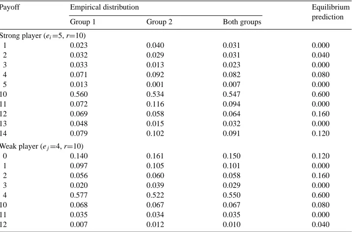
Table 6 presents the relative frequency distributions of payoff for the strong (upper panel) and weak (lower panel) players in Experiment 2. The format of the table is similar to Table 2. The realizable payoffs for the strong player are 1,2, . . . ,5,10,11, . . . ,14, and for the weak player they are 0,1, . . . ,4,10,11, and 12. The observed relative frequencies for Group 1, Group 2, and across the two groups are presented in columns 2, 3, and 4, respectively. The equilibrium payoffs are shown on the right-hand column. With a single exception, all the comparisons that we conducted between observed and predicted statistics yielded non-significant results.
7.2. Strong players
Under equilibrium play by both players, the expected payoff of the strong player is r=10. The mean payoff earned by the players in Group 1 (9.49) does not differ significantly from the theoretical value (z=1.42, p>0.07). A similar result holds for Group 2 (mean=9.29, z=1.90,
p>0.05). The variance of the payoffs under equilibrium play is equal to 8. We find again that
the observed variances do not differ from the theoretical value (10.15 (χ2=100.2, p>0.1) for Group 1; 10.88 (χ2=107.398, p>0.1) for Group 2). The relative frequency distribution of payoffs combined across both groups does not differ from the equilibrium probability distribution (Kolmogorov–Smirnov D160=0.094, p>0.1). The same result holds for each
of the two groups considered separately (D80=0.083, p>0.2, for Group 1, and D80=0.104, p>0.2, for Group 2).
7.3. Weak players
Table 6
Aggregate distribution of payoff in the asymmetric casea
Payoff Empirical distribution Equilibrium
prediction
Group 1 Group 2 Both groups
Strong player (ei=5, r=10)
1 0.023 0.040 0.031 0.000
2 0.032 0.029 0.031 0.040
3 0.033 0.013 0.023 0.000
4 0.071 0.092 0.082 0.080
5 0.013 0.001 0.007 0.000
10 0.560 0.534 0.547 0.600
11 0.072 0.116 0.094 0.000
12 0.069 0.058 0.064 0.160
13 0.048 0.015 0.032 0.000
14 0.079 0.102 0.091 0.120
Weak player (ej=4, r=10)
0 0.140 0.161 0.150 0.120
1 0.097 0.105 0.101 0.000
2 0.056 0.060 0.058 0.160
3 0.020 0.039 0.029 0.000
4 0.577 0.522 0.550 0.600
10 0.068 0.067 0.067 0.080
11 0.035 0.034 0.035 0.000
12 0.007 0.012 0.010 0.040
aThe relative frequencies were computed using the payoffs obtained over 80 trials. Nine subjects in each group were assigned the strong position (ei=5) in the first 80 trials and weak position (ej=4) in the second 80 trials;
another nine players were assigned the weak position in the first 80 trials and the strong position in the last 80 trials.
value (z=0.858, p>0.2, for Group 1, and z=1.162, p>0.12, for Group 2). Similarly, the variances of the observed payoffs — 7.91 and 8.52 for Group 1 (χ2=78.07, p>0.2) and Group 2 (χ2=84.16, p>0.2) — do not differ from the theoretical value. But the relative frequency distribution of payoffs combined across both groups differs significantly from the predicted distribution (D160=0.131, p<0.01). The significant difference is mainly due to
the payoffs earned by Group 2 (D80=0.146, p<0.01). The difference between the theoretical
and observed distributions for Group 1 is not significant (D80=0.117, p>0.2).
7.4. Strategy profiles
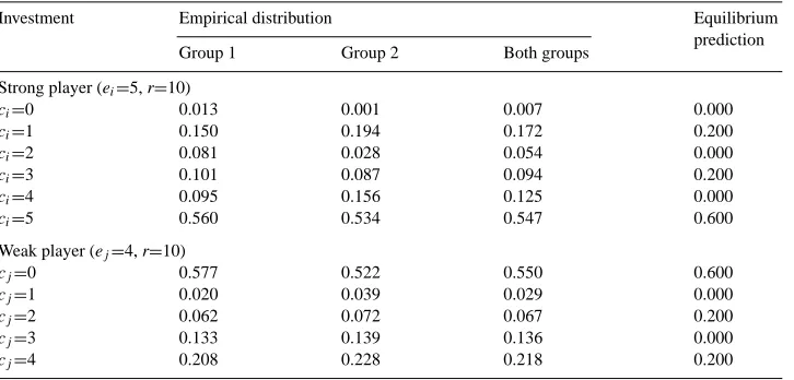
Table 7 shows the relative frequencies of choice of the investment strategies for the strong (upper panel) and weak (lower panel) players. In each case, the relative frequencies are summed across order of play. Also presented in Table 7 are the equilibrium probabilities of choice for risk-neutral players (computed from Eqs. (5)–(6)).
The weak players in Experiment 2 did not always play their minimax strategy; rather, across subjects, strategy cj=0 was played 55.0 per cent of the time by the weak players. The
Table 7
Aggregate distribution of investment in the asymmetric case
Investment Empirical distribution Equilibrium
prediction
Group 1 Group 2 Both groups
Strong player (ei=5, r=10)
ci=0 0.013 0.001 0.007 0.000
ci=1 0.150 0.194 0.172 0.200
ci=2 0.081 0.028 0.054 0.000
ci=3 0.101 0.087 0.094 0.200
ci=4 0.095 0.156 0.125 0.000
ci=5 0.560 0.534 0.547 0.600
Weak player (ej=4, r=10)
cj=0 0.577 0.522 0.550 0.600
cj=1 0.020 0.039 0.029 0.000
cj=2 0.062 0.072 0.067 0.200
cj=3 0.133 0.139 0.136 0.000
cj=4 0.208 0.228 0.218 0.200
row 5 (ci=5) each should be chosen 60 per cent of the time by risk-neutral weak and strong
players, respectively. Table 7 shows that, indeed, cj=0 was chosen by the weak player
almost exactly as often as ci=5 by the strong player, and that both were chosen slightly less
frequently than predicted. This discrepancy from equilibrium cannot be accounted for by risk aversion, because when u(x) is strictly concave, the strong player should, indeed, invest his entire capital less often than predicted, but the weak player should invest zero capital more often than predicted.
The frequencies of choice of the investment strategies by the strong players support the equilibrium solution. The relative distribution of frequencies combined across both groups does not differ significantly from the predicted distribution (D160=0.073, p>0.2).
We fail to reject the null hypothesis when the results of each group are considered sepa-rately (D80=0.056, p>0.2, for Group 1, and D80=0.090, p>0.2, for Group 2). However, the
frequencies of choice of the weak player do not support equilibrium play. When combined across both groups, the relative frequency distribution of strategy choices differ from the theoretical prediction (D160=0.153, p<0.01). The same significant discrepancy between
observed and theoretical distributions is obtained for each of the two groups separately (D80=0.140, p<0.05, for Group 1, and D80=0.167, p<0.05, for Group 2).8
Table 7 shows that row 0 (ci=0), column 1 (cj=1), and row 2 (ci=2) were chosen
very infrequently (0.007, 0.029, and 0.054, respectively). Iteratively dominated strategies occupying a higher position in the deletion hierarchy were chosen more frequently: column 3 (cj=0) and row 4 (ci=0) were chosen 13.6 and 12.5 per cent, respectively. These results
8The random matching of subjects undermines, though does not completely eliminate, the possibility of correlated strategies. We conducted another experiment identical to Experiment 2 in all details of the design with the only difference of using fixed pairs for all 80 trials of each phase rather than matching them randomly on each trial. The results of this experiment, which we plan to report elsewhere, were quite different. We observed many fixed pairs slowly converging to the pair of pure strategies in which the strong player invests ci=eiand the weak player
suggest that strongly dominated strategies, which should be iteratively deleted later in the sequence, were chosen more often than strategies that should have been deleted earlier. We shall test this hypothesis on the individual level later.
7.5. Trends in investment
We divided the 80 trials in each phase of the game into 8 blocks of 10 trials each. Then, for each weak player, we counted the number of times she invested 0 units in each block, denoted by f0, and for each strong player, the number of times he invested 5 units in each block,
denoted by f5. Table 8 presents the mean proportion of trials in which 0 units were invested
by the weak players and 5 units by the strong players. This information is presented by group, order of play, and block. Subjects who had played the role of the strong player in Phase 1 increased the frequency of 0 units investment in Phase 2, when assigned the role of a weak player. Whereas the mean proportion of 0 units investment across groups in Phase 1 was 0.49, the same mean proportion increased to 0.61 in Phase 2. The upper panel of Table 8 also shows that the order of play effect was stronger in Group 1 than in Group 2. The order of play effect was relatively steady across blocks in Group 1, but in Group 2, the effect was reversed after about 40 trials. Next, the lower panel of Table 8 shows that the subjects experiencing the role of weak player in Phase 1 decreased the frequency of investing 5 units in Phase 2 when assigned the role of the strong player. However, this effect was only manifested in Group 2.9
7.6. Individual differences
Fig. 3 displays the frequency distributions, one for each player role, of the number of trials in which 0 units (weak players) or 5 units (strong players) were invested by individ-ual subjects in the 80 iterations of the stage game. The distributions are computed across both groups and orders of play. Fig. 3 displays widely dispersed distributions with a com-mon mode at the frequency class 51–60. A comparison of the two distributions by the Kolmogorov–Smirnov test for two independent samples shows no significant difference
9To test for the effects of group, order of play, and block, the frequencies of choice f0and f5were subjected to a 2×2×8 group by order of play by block ANOVA with repeated measures on the group and block factors. Two separate ANOVAs were conducted, one for the weak players and the other for the strong players.
As for the weak players, the order of play main effect (F1,2848=33.5, p<0.0001), order of play by group interaction effect (F1,2848=7.5, p<0.006), order of play by block interaction effect (F7,2848=2.95, p<0.005), and the triple interaction effect (F7,2848=3.1, p<0.003) were all significant. Neither of the other main or interaction effects, none involving the order of play factor, were significant. The presence or absence of experience in playing the other role for 80 trials was the major factor causing subjects in the weak role to change the proportion of zero units investment. Although we have found no significant main effect due to group in Experiment 2, this result is qualified by the significant two- and three-way interaction effects involving group. As we noticed in Experiment 1, we have additional evidence that groups develop their own dynamics of play, and that switching opponents from trial to trial may not be sufficient to remove this ‘population’ effect.
Table 8
Experiment 2: mean relative frequency of trials in which 0 (weak players) or 5 (strong players) were invested Group Order Block
1 2 3 4 5 6 7 8 Mean
Weak playersa
1 W, S 0.52 0.51 0.34 0.53 0.42 0.46 0.49 0.50 0.47
1 S, W 0.64 0.73 0.66 0.63 0.78 0.72 0.68 0.61 0.68
2 W, S 0.41 0.43 0.36 0.48 0.66 0.49 0.67 0.53 0.50
2 S, W 0.67 0.59 0.56 0.44 0.54 0.59 0.46 0.49 0.54
Total 0.56 0.57 0.48 0.52 0.60 0.56 0.57 0.53 0.55
Strong playersb
1 S, W 0.47 0.54 0.53 0.51 0.63 0.60 0.63 0.56 0.56
1 W, S 0.60 0.56 0.59 0.60 0.57 0.51 0.53 0.53 0.56
2 S, W 0.49 0.41 0.49 0.67 0.62 0.57 0.62 0.72 0.57
2 W, S 0.53 0.44 0.41 0.51 0.53 0.48 0.54 0.50 0.49
Total 0.52 0.49 0.51 0.57 0.59 0.54 0.58 0.58 0.55
a0 units were invested. b5 units were invested.
between them (p>0.1). Recall that the equilibrium prediction of investing 0 units by the weak players or 5 units by the strong players in 80 trials is 0.6×80=48. Using the normal approximation to the binomial distribution (with a significance level set at 0.01), we tested the equilibrium prediction with the individual data. The null hypothesis was rejected for 22 of the 36 weak players and 18 of the 36 strong players.
7.7. Sequential dependencies
First-order sequential dependencies were assessed on the aggregate level, as in Exper-iment 1, by computing transition matrices of joint frequencies of choice on trials t and
t+1 across subjects and trials. As the transition matrices are very similar to the ones pre-sented in Table 5, they are omitted. Basically, they exhibit the same repetition bias as observed earlier. In particular, for the weak players, p(cj ,t+1=0|cj ,t=0)=0.72, whereas p(cj ,t+1=0|cj ,t=m) was equal to 0.27, 0.31, 0.21, and 0.40, for m=1, 2, 3, and 4,
respec-tively. For the strong players, the conditional probability of investing all the endowment was p(ci ,t+1=5|ci ,t=5)=0.72, whereas p(ci ,t+1=5|ci ,t=m) was equal to 0.33, 0.38, 0.32,
0.33, and 0.11, for m=4, 3, 2, 1, and 0, respectively. Similar results were obtained on the individual level. In essence, the subjects in Experiment 2, regardless of their role, exhibited the same strong repetition bias as in Experiment 1.
7.8. Iterative elimination of strictly dominated strategies
Fig. 3. Experiment 2: frequency distribution of the number of times: (A) 0 units (weak players); (B) 5 units (strong players) were invested.
However, as stated earlier, to justify deleting column 1 the weak player has to know that the strong player will not choose his strongly dominated row 0 (ci=0). Similarly, to justify
deleting row 2, the strong player must assume that the weak player will delete column 1 (cj=1). In other words, player i has to know that player j knows that player i will not play
his strongly dominated strategy.
that can not be satisfied by boundedly rational players. But when the number of pure strategies is relatively small, the full force of the common knowledge assumption is no longer needed. Event E is said to have knowledge level of degree 1, if player i knows it, of degree 2, if player j knows that player i knows it, of degree 3, if player i knows that player j knows that player i knows it, and so on. The ‘hierarchy of knowledge of rationality’ hypothesis states that the proportion of players with knowledge level of degree d decreases in d. When applied to our game, this hypothesis implies that some fraction of the subjects iteratively delete d strongly dominated strategies, a smaller fraction delete d+1 strongly dominated strategies, and so on.
Indirect support for this hypothesis has already been presented in Table 7. Under equi-librium play, row 0 (ci=0), column 1 (cj=1), row 2 (ci=2), column 3 (cj=3) and row 4
(ci=4) should have been iteratively deleted in this order. Table 7 shows that they were in
fact deleted on 99.3, 97.0, 94.6, 86.4, and 87.5 per cent, of all the trials, respectively. The hypothesis about hierarchy of knowledge of rationality predicts the sign of all 10 pair-wise differences between the five levels of d. Of these 10 predictions, nine are supported by the data. Only the difference between levels 4 and 5 is not significant (t=−1.23, p>0.1). Note that these are aggregate results that may mask considerable individual differences, whereas the hypothesis above refers to individual players.
To test the hierarchy of knowledge of rationality hypothesis on the individual level, we counted the number of subjects, out of 36, who chose any of the iteratively strongly dominated strategies on m occasions out of 80 trials. Table 9 presents the results. It shows that 32 of the 36 strong subjects always (on 80 out of 80 trials) deleted row 0. Further, 23 of the 36 weak players always deleted column 1. Table 9 also shows the number of subjects who erroneously chose any iteratively strongly dominated strategy no more than four times (5 per cent of the 80 decisions). If we allow for four ‘errors’ in a total of 80 rounds of play, then the majority of the subjects reveal four levels of iterated dominance (the exact frequencies are 34, 31, 26, and 19). Using this fairly strong criterion, 13 of the 36 subjects reveal five levels of iterated dominance. These results are significantly stronger than the ones reported in the different variants of the Beauty Contest game.
Subjects who approach the Investment game strategically, reason about their opponents’ decisions, and grasp the principle of IESDS, should iteratively eliminate strongly domi-nated strategies whether they play the role of strong or weak player. By switching roles
Table 9
Experiment 2: number of subjects choosing iteratively strongly dominated strategies (m times out of 80 trials) Strongly dominated strategies
m ci=0 cj=1 ci=2 cj=3 ci=4
0 32 23 6 11 3
1 2 3 7 4 5
2 0 2 6 2 0
3 0 2 2 0 4
4 0 1 5 2 1
5+ 2 5 10 17 23
after 80 trials, Experiment 2 was specifically designed to test this hypothesis. To test the hierarchy of knowledge of rationality hypothesis across both player roles, we counted for each subject the number of times, out of a total of 160 trials, that he or she played each of the following tuples of iteratively strongly dominated strategies: (row 0), (row 0 and column 1), (row 0, column 1, and row 2), (row 0, column 1, row 2, and col-umn 3), and (row 0, colcol-umn 1, row 2, colcol-umn 3, and row 4). The proportions of sub-jects who played these tuples no more than eight times (5 per cent of 160 trials) were 0.972, 0.889, 0.772, 0.500, and 0.194, respectively. These results strongly support the hy-pothesis about a hierarchy of levels of knowledge of rationality, showing that the ma-jority of the subjects, regardless of their role, engage in up to four dominance iteration steps.
8. Discussion
The equilibrium solution for the asymmetric Investment game has two major implica-tions. The first implication is that only iteratively undominated strategies will be chosen. Although this implication does not presuppose communality of beliefs or the same atti-tude to risk, it may still impose strong demands on the players’ cognitive system when the number of iteratively dominated strategies is large. Evidence from sequential bargaining experiments (e.g., Roth, 1995b), Centipede game (McKelvey and Palfrey, 1992), and the Beauty Contest game suggests that subjects typically do not use backward induction for iter-atively deleting strongly or weakly dominated strategies even if the number of stages in the game is limited and small. Our data support a bounded process of IESDS, which postulates a hierarchy of classes of players who differ from one another in their level of knowledge of rationality.
9. Adaptive learning
Our purpose in the present section is to account for the major patterns of results in Experiments 1 and 2 by the ‘experience-weighted attraction’ (EWA) learning model that was recently proposed by Camerer and Ho (1999), and subsequently tested experimentally on different sets of data (Camerer and Ho, 1998, 1999). We chose the EWA model because it has three desirable properties. Firstly, it satisfies the three principles of actual, simulation, and declining effects. The first principle, shared by all reinforcement-based models, states that successes increase the choice probability of chosen strategies. The second principle asserts that unchosen strategies, which would have yielded high payoffs, are more likely to be chosen in the future. The third principle states that, with experience, players move to reduce discrepancies between actual and foregone payoffs. Secondly, the EWA model contains both belief-based (e.g., Fudenberg and Levine, 1998) and reinforcement-based (e.g., Roth and Erev, 1995) learning models as two special cases. Thirdly, the EWA model captures interactive decision situations in which players use information about their own payoffs together with information about the history of play by their opponents in adjusting their choice behavior. These three properties render the EWA model especially suitable to account for the dynamics of play in our two experiments, which seem to combine elements of reinforcement (the sequential dependencies reported in both experiments) and beliefs (the deletion of strongly dominated strategies in Experiment 2). We make no attempt to compare the EWA model with alternative learning models (e.g., Fudenberg and Levine, 1998). Rather, we have a more modest purpose of using this model to account for some of the major behavioral regularities that were reported in Sections 4 and 7.
9.1. The EWA learning model
At the heart of the EWA model are two parameters that are updated after each round of play. The first parameter, denoted by N(t), is interpreted as the number of observations-equivalents of past experience. The second parameter, denoted byAcm
k (t ), is interpreted
as the attraction of investing m units by player k after round t. The initial values of these two parameters are denoted by N(0) andAcm
k (0). For updating N(t), the model assumes that N(t)=ρN(t−1)+1, t≥1, where the parameterρ(0≤ρ≤1) is the rate of depreciation. While updating the attraction of a strategy, payoffs corresponding to unchosen strategies are given a weight ofδ, whereas the payoffs pertaining to chosen strategies are given additional weight of 1−δ. Previous attractions are depreciated by another parameterφ(0≤φ≤1). Earlier, we used ck=m to denote the strategy of investing m (m=0, 1, 2, 3, 4, 5) units by player k (k=i, j). To be consistent with Camerer and Ho (1999), hereafter we denote strategy ck=m by scm
k . The attraction of strategys cm
k , namelyA cm
k (t ), is a weighted average of the payoff for
period t and the previous attractionAcm
k (t−1):
In the above expression, I(x, y) is an indicator variable which equals 1, if x=y and 0, if x6=y,
when,δ=0,ρ=0, and N(0)=1, the attractionAcm
k (t )resembles the reinforcement of classical
reinforcement-based learning models. Ifδ=1 andρ=φ, then the attraction corresponds to updated expected payoffs as in belief-based learning models.
Having briefly described the attraction of choosing to invest ckon trial t,Ackm(t ), we
pro-ceed to define the probability of player i investing ck on trial t+1 by the Logit
function:
pcm
k (t+1)=
eλAcmk (t )
Pek
l=1e λAclk(t ),
where the parameterλmeasures sensitivity of the players to attractions.
10. Results
The model parameters for each of the two experiments were estimated by the maximum likelihood method.
10.1. Experiment 1
We estimated separately the model parameters for Games L and H. The estimated pa-rameter values and measures of goodness of fit for the EWA model (column 3) and for each of its two special cases — the reinforcement-based (column 4) and belief-based (column 5) models are presented in Table 10.
10.2. Overall model fit
Table 10 shows that, as expected, the hybrid EWA model outperforms both the rein-forcement-based and belief-based learning models in tracking the investment behavior of the subjects in both Games L and H. This is affirmed by the goodness of fit statistics of log-likelihood ratio, Akaike Information Criterion (AIC), Bayesian Inference Criterion (BIC), andχ2(p<0.00001), all four of which are reported in Table 10. The reinforcement-based learning model outperforms the belief-reinforcement-based model, and is in turn slightly outper-formed by the EWA model. Note that the reinforcement-based model hypothesizes that the player’s decision depends on the sum of past payoffs. Whereas, the EWA model parameter estimates support the hypothesis that decision depends on the average of past payoffs. The reported parameter estimates are significant (α=0.01).
Using a similar format to Table 3, Table 11 presents the EWA model predictions of the choice probabilities in Game L (top panel) and H (second panel). The EWA model clearly over-estimates the choice probability of investing the entire resource (ci=5) in
Table 10
Estimation of learning model parameters: Experiment 1
Parameter Model
EWA Reinforcement-based Belief-based
Reward condition: low reward (r=8)
δ 0.000 0.000 1.000
Log-likelihood −3551.70 −3563.76 −4649.39
AIC −3560.70 −3569.76 −4656.39
BIC −3587.55 −3587.65 −4677.27
ρ2 0.310 0.308 0.098
χ2 24.111 2195.386
(p-value, d.o.f) (0.00003) (0.00002)
Reward condition: high reward (r=20)
δ 0.000 0.000 1.000
Log-likelihood −2908.08 −2928.29 −3634.02
AIC −2916.08 −2933.29 −3640.02
BIC −2939.94 −2948.20 −3657.92
ρ2 0.435 0.431 0.295
χ2 40.416 1451.890
(p-value, d.o.f) (0.00003) (0.00002)
aParameter estimates are significant (α=0.01).
sequential dependencies observed in Experiment 1. The first-order sequential dependency in investing the entire resource is predicted by EWA model to be 0.974, whereas the observed sequential dependency in this case is 0.65 (Table 5).
Table 11
EWA model predictions of investment choices: Experiments 1 and 2a
Investment Predicted distribution Observed
behavior
Group 1 Group 2 Both groups
Experiment 1, Game L: low reward condition (e=5, r=8)
ci=0 0.078 0.216 0.147 0.169
ci=1 0.070 0.069 0.069 0.116
ci=2 0.083 0.048 0.065 0.088
ci=3 0.048 0.113 0.081 0.118
ci=4 0.060 0.047 0.054 0.090
ci=5 0.662 0.507 0.584 0.418
Experiment 1, Game H: high reward condition (e=5, r=20)
ci=0 0.062 0.030 0.046 0.141
ci=1 0.034 0.010 0.022 0.055
ci=2 0.036 0.036 0.036 0.053
ci=3 0.000 0.000 0.000 0.053
ci=4 0.002 0.066 0.034 0.069
ci=5 0.866 0.858 0.862 0.628
Experiment 2, weak player (e=4, r=10)
cj=0 0.808 0.745 0.777 0.550
cj=1 0.000 0.014 0.007 0.029
cj=2 0.002 0.050 0.026 0.067
cj=3 0.090 0.110 0.100 0.136
cj=4 0.100 0.081 0.090 0.218
Experiment 2, strong player (e=5, r=10)
ci=0 0.000 0.000 0.000 0.007
ci=1 0.113 0.159 0.136 0.172
ci=2 0.035 0.007 0.021 0.054
ci=3 0.060 0.020 0.040 0.094
ci=4 0.018 0.082 0.050 0.125
ci=5 0.775 0.732 0.754 0.547
aThe right-hand columns show the relative frequencies computed using the observed investment decisions of Groups 1 and 2 in Experiments 1 and 2 (refer to Tables 3 and 7).
to the observed probabilities of 0.662 and 0.594. Similarly, the predicted probability (0.99) of sequential dependency in investing the entire capital exceeds the observed probability of 0.79 (Table 5).
10.3. Pre-game disposition
10.4. Interpretation of the parameter values
As the estimated value ofδ is 0 in both Games L and H, we can infer that the choice of strategies in these games was not guided by expected payoffs. Rather, the investment decisions were based on the payoffs earned in previous trials. In particular, the choice of strategies was not based on beliefs about the likely actions of competitors. The estimates of the parametersφandρare equal in both games, implying that the average of past payoffs, rather than the sum of past payoffs, guided the choice of the investment strategy. Finally, the estimates of the sensitivity parameterλ(Game L: 0.755; Game H: 0.967) suggest that the subjects paid attention to the likely reward on winning the competition.
10.5. Experiment 2
Table 12 reports similar results for Experiment 2. As in Experiment 1, we find that the EWA model outperforms both the reinforcement-based and belief-based models. Specifi-cally, the EWA model fits the data better than the reinforcement-based (χ2=178.1, p<0.001) and belief-based (χ2=1413.5, p<0.001) learning models. The AIC and BIC support this inference. The parameter estimates are significant (α=0.01).
The lower two panels of Table 11 present the distribution of strategies predicted by the EWA model for the weak and strong players. The model tends to over-predict the investment of the entire capital by the strong players (0.754 versus 0.574) and zero investment by the weak players (0.777 versus 0.550). Quite interestingly, the EWA model predicts the deletion of dominated strategies, namely, strategies ci=0, cj=1, ci=2, cj=3, and ci=4,
in proportions that closely approximate the actual choices of the subjects. Table 11 shows that the strategies ci=0, cj=1, ci=2, cj=3, and ci=4 were predicted to be deleted 100,
99.3, 97.9, 90.0, and 95.0 per cent of the time across subjects. The EWA model predictions compare favorably with the actual percentages of deletion (obtained by subtraction), namely, 99.3, 97.1, 94.6, 86.4, and 87.5. In a manner similar to Experiment 1, the EWA model over-estimated the magnitude of the sequential dependencies. For instance, the EWA model predicts p(ci ,t+1=5|ci ,t=5)=0.97 and p(cj ,t+1=0|cj ,t=0)=0.98 compared to the observed
result of 0.72.
10.6. Pre-game disposition
Supposedly through introspection, the strong players had eliminated the option of in-vesting 0 (A0(0)=0) before the experiment commenced. But they did not eliminate the other two dominated strategies, namely, ci=2 and ci=4 (A2(0)=7.432; A4(0)=9.188). At
the commencement of the game, the strong players were strongly disposed toward in-vesting all their capital (A5(0)=11.681). However, the strength of this predisposition, as indicated by the estimate N(0)=1.418, is less than the experience derived from playing two trials.
In the bottom panel of Table 12, we notice that weak players were able to eliminate the second level of dominated strategy, namely cj=1 (A1=0). There is some theoretical support
for elimination of the dominated strategy cj=3 by introspection, as the corresponding