CNR-CACOH, Lyon, France [email protected]
Commission VI, WG VI/4
KEY WORDS: drone, metrology, bowl effect, drift, dyke, MicMac, 4D monitoring
ABSTRACT:
The photogrammetric treatment of images acquired on a linear axis is a problematic case. Such tricky configurations often leads to bended 3D models, described as a bowl effect, which requires ground measurements to be fixed. This article presents different solutions to overcome that problem. All solutions have been implemented into the free open-source photogrammetric suite MicMac. The article presents the lasts evolutions of MicMac's bundle adjustment core, as well as some extended calibration models and how they fit for the camera evaluated. The acquisition process is optimized by presenting how oblique images can improve the accuracy of the orientations, while the 3D models accuracies are assessed by producing a millimeter accurate ground truth from terrestrial photogrammetry.
1. INTRODUCTION
Unmanned Aerial Vehicles (UAV) have been stubbornly standing as a trendy topic. By embarking a consumer grade camera on a small UAV, it is possible to photograph a site to organize its surveillance. On the other hand, the photogrammetrist and computer vision communities have been working closer. A high automation degree has been reached, such as many software can turn automatically a set of pictures into a visually good looking 3D model. The combination of both technologies is very promising, but still faces challenges (Remondino et al., 2011).
Compagnie Nationale du Rhône (CNR), a hydraulic energy producer and the concessionary of the Rhône river, set up a partnership with IGN, the French Mapping Agency, to organize a metrological monitoring of its dykes. Such linear structures are problematic for the 3D reconstruction using photogrammetry, as they engender what is described in (James et al., 2014) as a bowl effect.
The objective is to acquire images using light and low-cost aerial means, and to produce 3D models with an accuracy within one centimeter. By comparing 3D models acquired at different times, the industrial wishes to detect early signs of possible weakness in its dykes, and prevent further damages. This paper aims to present a method than can be used to assure a very fine accuracy on linear work, and that minimizes the amount of Ground Control Points (GCP) required - one for each 100 meters long. Photogrammetric treatment are done through MicMac, the free open-source photogrammetric suite developed at IGN, in which all the evolutions presented have been implemented. A typical workflow describes the procedure in the Appendix.
After a presentation of the acquisitions and the advantages of using UAV photogrammetry instead of other technologies, the article focuses on the problematic image processing. The improvements integrated into MicMac's bundle adjustment core will be presented.
In the second part, extended calibration models will be introduced and their interest assessed. A three step auto calibration process is proposed to minimize Check Points (CP) reprojection errors before any compensation on the GCP, in
which a non radial correction is stacked over a radial camera model.
An innovative way to correct external orientations from GCP is presented. Finally, some accuracy assessment and results are exposed to demonstrate the effectiveness of the solution.
2. DATASETS
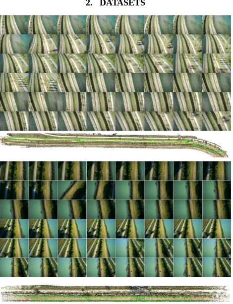
Figure 1: Both datasets are made of a mix of vertical and oblique images, acquired on two parallel strips. 2015 acquisition (up) overlaps the 2014 (down)
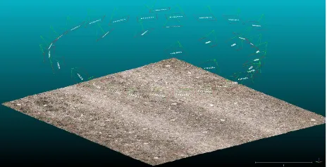
Figure 2: Perspective view over a ground control zone (GCZ) and the 35 images acquired to produce it
La Palliere's dyke is a structure subject to a reinforced monitoring. Visual surveillance, combined to topographic leveling and piezometric measurements are deployed to monitor a subsidence zone. The 1200 meters long structure has been used as a test site, on which two acquisitions have been conducted, in 2014 (only 600 meters long) and 2015 with a nine months interval between each.
Each dataset is made of an Unmanned Aerial Vehicle (UAV) acquisition, 45 GCP and 10 Ground Control Zones (GCZ), both evenly distributed along the profile. A GCZ is a roughly 2x2 meters rectangular area, delimited by 5 GCP, and on which terrestrial images have been acquired to produce a millimeter accurate ground truth.
The UAV acquisition has been realized with a rotary wing UAV, embarking a Sony DSC-RX1. Two parallel axis have been realized, with a transverse and longitudinal overlap of 80%. By flying at 60 meters high, the resulting vertical images have a resolution of 1 cm. Oblique images have been acquired with the same flight plan, the gimbal tilted at 45°.
French authorities have set standards governing the use of civilian UAVs. As a result, four flying scenarios have been created, with a growing complexity of use and certification. The first scenario is the most simple to access, it requires the pilot to remain within 100 meters from its UAV. Therefore multiple flights can added from after another, and the complete survey can be done in 6 flights, requiring around two hour.
The most time-consuming task is about setting up and surveying the GCP. While many research focus on integrating RTK-GNSS receiver on these platforms (Stempfhuber et al., 2013, Jones et al., 2014), this work focuses on how to minimize the amount of GCP required by applying a proper photogrammetric treatment.
3. DATA PROCESSING
3.1 Bowl effect
Critical configurations have been the recent object of multiple studies (Nocerino et al., 2013, Nocerino et al., 2014, James et al., 2014, Wu, 2014). These studies have shown that the photogrammetric treatment of linear acquisitions can be problematic. By leading to a bad estimation of the camera's internal parameters, the result is an inaccurate 3D model requiring many ground measurements to be fixed.
The MicMac suite has been used for all the following results. It integrates, via the Tapas interface, five classical distortion models (Table 1). After a tie point automatic detection based on (Vevaldi, 2010) C++ Sift implementation, with images subsampled by a factor 4, the orientations of vertical images have been determined by using each camera model alternatively. Before any compensation on the GCP, the orientations accuracies can be assessed by analyzing the evolution of the reprojection error along the dyke. When using improper camera model and a poor network made of vertical images, the estimated set of orientations can be bended, which is described in the literature as a bowl effect, and illustrated by Figure 3.
Figure 3: Evolution of the altimetric reprojection error of check points along the profile, for different camera model applied on dataset 2015. The bowl effect is characterized by a parabolic drift of the resulting orientations. Different calibration models implies different drifts, which are minimized for the camera tested by using the most complex characterization of the optical deformations.
To correct this drift, two strategies are possible : • set up, survey, and use ground measurement; • improve of the aerotriangulation estimation.
Depending on the accuracy targeted, the first option might imply a high amount of field work. However a high drift will require a lot of measurements to be fixed. Their amount and distribution along the profile are not easy to forecast. It is also not always possible, as working with historical images, or when the UAV surveys a structure inaccessible from the ground. The improvement of the bundle adjustment is a solution that combines all the advantages.
3.2 MicMac's bundle adjustment evolutions
Bundle block adjustment is the problem in which the positions and orientations of a set of cameras are determined from a set of homologous points. As a non linear problem, it can be solved by iterations of the least-square method, in which a cost function quantifying the gap between bundles is minimized (Pierrot-Deseilligny, 2011).
A first couple of images is oriented using the essential matrix algorithm, or more probably the space resection algorithm if there is a sufficient amount of homologous points. Including an initial basic camera model, images are added by small groups, following an optimal tree built along a criteria giving advantage to the stability to avoid divergences.
Once the whole set of images is oriented, the camera model is released and the unknowns of calibration appear as unknowns in the least square problem. Iterations are done to minimize the solution until the convergence is reached.
Until mid 2014, the convergence was reached after a fixed amount of iterations that could be defined by experimented users. It is now considered reached when the ratio between d (the displacement in euclidean geometry of a homologous point reprojection between two iterations) and D (the depth of the scene) is lower than 1.10-10.
The Levenberg-Marquardt algorithm (Moré, 1978) is used to add a viscosity coefficient on the unknowns between the iterations. It helps to find solutions even if the initial values given to the unknown are far from the ground truth. The viscosity coefficient has to be determined properly :
• too high, it will lead to divergences; • too low, it will converge to a wrong solution.
Table 1: Description of the basic distortion models easily accessible in MicMac. Experimented users can define their own camera model as well as the way to liberate parameters in the bundle adjustment.
3.3 Combination of camera models
When looking closer at the details of each camera model, one can observe that, for the camera tested, the altimetric drift is minimized when :
• a center of distortion is calculated, distinct from the center of perspective;
• a high degree polynomial radial correction is applied; • a decentric and affine correction is applied.
Given these observations, it is interesting to apply additional degrees to the radial correction. Moreover, an extra calibration layer is added by stacking a non radial polynomial correction to rectify the deformations that have not been corrected by the previous steps. A three-steps calibration process is applied in which :
1. A first basic model is calculated on a 10 images subset, to get a physical description of the description; 2. Using the first model as an initial value on the whole dataset, extra polynomial coefficients are added to improve the description of the optical deformations; 3. A non radial polynomial correction is added to rectify
the deformations left
The first model describes the basic physical geometry of the camera. It considers PPA and PPS equals, and applies a radial correction dR1 : R = distance between a pixel and the PPS
The second step refines previous calculation. For the camera tested, it is better to distinguish PPA from PPS, add an affine and a decentric correction, and it applies a radial correction
A third step is realized by stacking an extra layer, made of a purely mathematical model, as described in (Tang et al., 2012) and (Jacobsen, 2007). It is made of the sum of all monomials and polynomials between 0 and 7 :
D(X,Y)=
∑
where X, Y = image coordinate
Table 2: Evolution of the reprojection error according to the camera model (working only with the vertical images). The table shows that, for the camera tested, a combination of extended camera models is preferable.
The step by step approach is necessary to limit the risk of over-parametrization. Due to the amount of parameters to determine, the amount of computing time is higher, although many refinements are possible to meet with the user's specific need.
3.4 Inclusion of oblique images
The nature of dykes is problematic in the case of auto-calibration. The difference in height between the highest and the lowest point is small, such as the scene can be seen as planar. According to the literature (Triggs, 1998, Fraser, 1987), it is recommended to realize a specific acquisition : a high number of images (at least 10), and an angular spread between cameras of at least 10 to 20°.
The high repeatability is achieved by fixing a high overlap (80%) and by flying on two parallel strips. On average, each point is seen in 10 vertical images, and the maximum angle spread between cameras is 19°.
By adding oblique images with the same flight plan, but tilted with an angle of 45°, each point is seen in at least 20 images, and the angle spread can reach 90°.
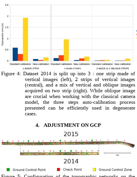
These last conditions are highly favorable for a better auto-calibration of the lens distortions. As Figure 4 expresses, the reprojection errors are disproportionately lower when oblique images are used. Interestingly, the auto-calibration process presented in the previous part presents satisfying results even in the most degenerate configuration.
In certain datasets with favorable networks, it is probably better to use a physical camera model. The determination of many additional parameters can lead to an over-parametrization of the least-square estimation. In these cases, the user should avoid applying the last layer of calibration - equation (3). These seem however efficient in degenerate cases as presented.
Figure 4: Dataset 2014 is split up into 3 : one strip made of vertical images (left), 2 strips of vertical images (central), and a mix of vertical and oblique images acquired on two strip (right). While oblique image are crucial when working with the classical camera model, the three steps auto-calibration process presented can be efficiently used in degenerate cases.
4. ADJUSTMENT ON GCP
Figure 5: Configuration of the topographic networks on the acquisitions
A set of relative orientations can be useful for visual purposes. In the cases studied, GCP are needed to georefence the site, and especially to overcome the remaining imprecision of the orientations.
For the georeferencement of a scene, a Helmert transformation can be done using three GCP visible in three images. A bended set of orientations will remain bended that way, which is problematic considering the recurrent twist observed in linear works.
A solution is to perform a bundle adjustment in which are included the image measurements of GCPs. As observations among the tie points, the difficulty of the problem is to find the proper weight :
• too low, the bowl effect will not be counterbalanced; • too high, the orientations will stick on the
measurements and create wavelets between these references.
Many experiments have been led to find the optimal parameters. However, no general correlation has been found on the different datasets. Although some characteristics seem to be efficiently applicable for all bundle adjustments with GCP :
• refine the calibration by letting it free (not valid for photogrammetric cameras);
• reject all tie points whose residual exceed one pixel; • weight tie points individually according to their
residuals to give advantage to the best ones. A weighting function W has been refined such as :
W
(
Ri)
= 1√
(
1+(
R i 0.2
)
2
)
(4)where i = a given tie point
Ri = residual for the tie point i in the bundle adjustment
Figure 6: Principle of the altimetric drift estimation by a polynomial. By using the reprojection error, a correction can be calculated
Another approach has been developed to match with the recurrent deformations observed. As the altimetric drift results from a misevalutation of the internal parameters, it creates a parabolic drift that can be estimated by a two degree polynomial. The determination is done by using the reprojection errors on GCP. A polynomial correction function P can be applied if :
P
(
J i)
=GiApplying a polynomial estimation of the drift on the Z axis, it turns into :
J
Zi+a+b.JXi+c.JYi+d.JXi
2
=G zi
which can be expressed as :
a+b.J
Xi+c.JYi+d.JXi2=Gzi−JZi (5)
where a, b, c, d= polynomial coefficients (real numbers) JXi, Jyi, Jzi = X, Y, Z reprojected coordinates for i GXi, Gyi, Gzi = X, Y, Z ground truth coordinates for i. Gzi- Jzi = altimetric reprojection error for i.
Equation 5 requires at least 4 GCP to be solved. The results achieved through that process are interesting (Figure 7). It has been tested on several datasets and is still under development. The primary conclusion is that the method seems efficient while working on relatively short linears. On the long ones, as the 1200 meters from dataset 2015, the process is not satisfying yet and needs further refinements. It is however very promising in terms of computing time, as a set of orientations can be adjusted after a few seconds, while the inclusion of GCP in the bundle adjustment requires a few hours with the dataset presented.
Figure 7: Comparison between three adjustment on GCP methods proposed : automatic (left) bundle adjustment with GCP, manual bundle adjustment with GPC, estimation of a polynomial correction
5. RESULTS
Figure 8: The regularization process estimates the difference in height between the pixel to evaluate and its neighbors. It usually smooths the blades of grass, tiny holes, but can also misevaluate a check points altitude.
Table 3: Dataset 2015, the 1100 meter long acquisition is calculated using different camera model. The results after compensation on 11 GCP confirms that an improper camera model is not efficiently corrected.
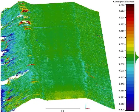
To bypass that issue, 10 GCZ have been spread along the field. With a submillimetric GSD, the resulting pictures have been turned into a millimeter accurate 3D model, converted into a mesh, and used as a ground truth. The pointcloud issued from the UAV acquisition is then compared to the mesh extracted on the GCZ.
Figure 9: Perspective view over the colored pointcloud derived from the 2015 UAV acquisition. The blue section highlights the 2014 acquisition
Figure 10: Dataset 2014: comparison between the mesh constructed from the terrestrial images, and the pointcloud derived from the UAV acquisition. Except for Z1, on the edge of the survey zone, these ground control zones present results in accordance with the 1cm on the altitude accuracy targeted The difference between both follow a normal distribution with millimetric indicators (Table 3). From these data, the accuracy at one (68,3%) and three sigmas (99,7%) can be estimated. Figure 10 shows the visual repartition of the comparison; it underlines how tricky a punctual check can be. Each little rock or blade of grass are modelized from the terrestrial acquisition, but not with the UAV dataset.
Table 4: Indicators qualifying the accuracy of both datasets according to the mesh to pointcloud comparison, in which the ground truth are GCZ with millimetric accuracies.
The purpose of this work being a better risk prevention in hydraulics works, a diachronic monitoring can be organized with these data. Many file format and specifications coexist : pointcloud, 3D mesh, grid,...
Figure 11: Perspective view over the comparison between the mesh triangulated from the 2014 model and the pointcloud from the 2015 campaign. The juxtaposition of 3D models illustrates that the highest changes happen on the slopes hit by the river or covered by nature. The central road seems stable, which is a good sign for the internal structure's health.
X [cm] Y [cm] Z [cm]
RadialBasic 2.5 2.4 9.4
RadialStd 0.9 0.6 2.8
RadialExtended 0.9 0.6 2.8
FraserBasic 0.8 0.5 2.1
Fraser 0.7 0.6 3,0
As demonstrated in (Boudon et al., 2015), the pointcloud to mesh comparison seems to be a good compromise between the computing time required, the analysis steming from the differences observed, and the existence of free open-source solutions such as CloudCompare (Girardeau-Montaut, 2006). A repeatability test had been led on the 2014 campaign, by acquiring two independent sets of images. After applying the same workflow on both datasets, the first 3D model has been turned into a pointcloud after compensation on 6 GCP, while the second one turned into a pointcloud after compensation using both GCP and CP (45 measurements). The comparison shows a normal distribution with the following indicators :
• mean distance : -5 mm • standard deviation : 35 mm
These indicators have to be nuanced acknowledging the distribution of these distances along the model. The highest differences are measured on the edges of the survey and on the slopes. A few remeshing issues also weakens the analysis. By narrowing the selection of the highest values, it is very possible the improve these within a few millimeters.
The technique however shows that it can be applied to detect changes in elevation within a few centimeters on large areas.
Figure 12: Repeatability test led on the 2014 acquisition. The test shows that the imprecision occur mostly on the areas covered with dense vegetation and on the edges.
6. CONCLUSION
The paper presented the problematic inherent to linear surveys. Such configurations often lead to a bad estimation of the camera's internal parameters, and thus degrades the accuracy of the solution, bending it along the depth of the scene.
The high accuracy required by industrials combined to the technical specifications of UAVs and their reduced payload limits the technical solutions applicable, and motivated the interest for the study.
A three step auto calibration process is presented in which a first model describes the physical parameters of the lens. Extended polynomials are used for the radial correction of the lens distortions. A third non radial correction is finally stacked. Made of a sum of monomials and polynomials, it is used to correct the deformation that have been corrected by the physical description estimated on the previous steps.
The inclusion of oblique images, object of multiple studies, has been confirmed as a powerful way to improve the accuracy of the orientations. It also underlines that the three-steps
calibration is powerful even in critical configurations, and especially when only one strip of vertical images is available. The orientations are then adjusted on GCP. Our experience proved that one GCP for each 100 linear meter can be enough to get most of CP's reprojection errors under one centimeter. Such data is used to generate 3D models and organize a 4D monitoring. As the structures studied are covered by nature (trees, grass,...) a very fine level of detail is achieved. Tiny changes can be detected, the difficulty is now to know when these changes are a sign of subsidence, and which recommendations should be given to the river concessionary.
ACKNOWLEDGMENTS
The authors would like to thank the Compagnie Nationale du Rhône for its participation in this research project. We are grateful to José Cali, lecturer and researcher at ESGT, as well as Jacques Beilin, lecturer and researcher at ENSG who both helped us through an underscale reproduction in a metrological environment to get a better understanding of these specific acquisitions.
Thank you also to the Aerial Activities Service from IGN, L'Avion Jaune, Redbird, and Vinci-Terrassement for their involvement in the aerial acquisitions.
Thank you finally to IGN's LOEMI engineers and researchers for their expertise with camera hardware and post-processing, and to IGN's Travaux Spéciaux, for their metrological skills.
REFERENCES
Boudon, R., Rebut, P., Mauris, F., Faure, P-H, Tournadre, V., Pierrot-Deseilligny, M., 2015. Actes du Vingt-Cinquieme Congrès des Grands Barrages, Stavanger (Norway), June 2015. Q. 99 – R.53, pp. 742-765.
Fraser, C.S., 1987. Limiting error propagation in network design in photogrammetry. Photogrammetric Engineering and Remote Sensing, Vol. 53(5), pp. 487-493.
Jacobsen, K., 2007. Geometric handling of large size digital airborne frame camera images. Optical 3D Measurement Techniques VIII, Zürich (Switzerland), pp. 164-171.
James, M. R., Robson, S., 2014. Mitigating systematic error in topographic models derived from UAV and ground‐based image networks. Earth Surface Processes and Landforms, 39(10), pp. 1413-1420.
Jones, K. H., & Gross, J., 2014. Reducing Size, Weight, and Power (SWaP) of Perception Systems in Small Autonomous Aerial Systems. In Proc. 14th AIAA Aviation Technol., Integration, Oper. Conf., Atlanta (USA).
Girardeau-Montaut, D., 2006. Détection de changement sur des données géométriques. Thesis manuscript, Telecom Paris, Paris (France).
Moré, J.J., 1978. The Levenberg-Marquardt algorithm: implementation and theory. Numerical analysis, pp. 105-116. Springer Berlin Heidelberg.
Nocerino, E., Menna, F., Remondino, F., Saler, R., 2013. Accuracy and block deformation analysis in automatic uav and terrestrial photogrammetry - lesson learnt. International Archives of Photogrammetry, Remote Sensing and Spatial Information Sciences, II-5/W1, pp. 203-208.
Pierrot-Deseilligny, M., Clery, I., 2011. Apero, an open source bundle adjusment software for automatic calibration and orientation of set of images. International Archives of the Photogrammetry, Remote Sensing and Spatial Information Sciences, 38, 5.
Remondino, F., & Fraser, C., 2006. Digital camera calibration methods: considerations and comparisons. International Archives of Photogrammetry, Remote Sensing and Spatial Information Sciences, 36(5), 266-272.
Remondino, F., Barazzetti, L., Nex, F., Scaioni, M., Sarazzi, D., 2011. UAV photogrammetry for mapping and 3d modeling– current status and future perspectives. International Archives of the Photogrammetry, Remote Sensing and Spatial Information Sciences, 38(1), C22.
Remondino, F., Del Pizzo, S., Kersten, T., Troisi, S., 2012: Low-cost and open-source solutions for automated image orientation – A critical overview. Proc. LNCS 7616, pp. 40-54.
Stempfhuber, W., 2013. 3D-RTK capability of single GNSS receivers. International Archives of Photogrammetry, Remote Sensing and Spatial Information Sciences. Volume XL-1/W2, pp 379-384.
Tang, R., Fritsch, D., Cramer, M., 2012. New rigorous and flexible Fourier self-calibration models for airborne camera calibration. ISPRS Journal of Photogrammetry and Remote Sensing, Volume 71, 76-85
Triggs, B., 1998. Autocalibration from planar scenes. In Proc. 5th European Conference on Computer Vision, pages 89–105, Freiburg (Germany).
Vevaldi, 2010. SIFT++ A lightweight C++ implementation of SIFT. http://www.robots.ox.ac.uk/~vedaldi/code/siftpp.html. Last access on June 15th 2015.
Wu, C., 2014. Critical configurations for radial distortion self-calibration. The IEEE Conference on Computer Vision and Pattern Recognition (CVPR), Columbus (USA), pp. 25-32.
APPENDIX
Here is presented for the interested MicMac users the workflow used to compute a 3D model using the workflow detailed in the article :
Detection & matching of homologous tie points using a multi scale approach (change 1500 into -1 if results are not satisfying)
• mm3d Tapioca MulScale “.*RAW” 400 1500 Description of the lens distortion by a basic camera model, on a small subset (10 images) of the whole dataset
• mm3d Tapas Four15x2 “DSC0005[0-9].RAW” DegRadMax=3 DegGen=0 Out=Calib1
Refinement of the previous model on the whole dataset, in which is added decentric and affine parameters, as well as the radial unknowns up to degree 15
Georeferencement and specific adjustment on GCP (image measurements in ImgMeasures-S2D.xml)
• mm3d GCPBascule “.*RAW” Relative Georef
GCP.xml ImgMeasures-S2D.xml
PatNLD=”RegEx_for_GCP” NLDegZ=[1,X,Y,X2] NLFR=false
OR classical use of GCP in the bundle adjustment
• mm3d Campari “.*RAW” Relative Georef GCP=[GCP.xml,1,ImgMeasures-S2D.xml,0.5] AllFree=true SigmaTieP=0.2
Computation of the depth map, orthophotography, and colored pointcloud
• mm3d Malt Ortho “.*RAW” Georef
• mm3d Tawny Ortho-MEC-Malt/
• mm3d Nuage2Ply MEC-Malt/NuageImProf_STD-Malt_Etape_9.xml Attr=Ortho-MEC-Malt/Ortho-Eg-Test-Redr.tif