Applications of geographical information
systems (GIS) for spatial decision support in
aquaculture
Shree S. Nath
a,*, John P. Bolte
b, Lindsay G. Ross
c,
Jose Aguilar-Manjarrez
daSkillings-Connolly,Inc.,5016 Lacey Boule6ard S.E.,Lacey,WA 98503, USA bDepartment of Bioresource Engineering,Oregon State Uni6ersity,Cor6allis,OR97331, USA
cInstitute of Aquaculture,Uni6ersity of Stirling,Stirling FK9 4LA, UK
dFood and Agricultural Organisation of the U.N,Viale delle Termi di Caracalla,00100 Rome, Italy
Received 1 September 1999; accepted 2 October 1999
Abstract
Geographical information systems (GIS) are becoming an increasingly integral component of natural resource management activities worldwide. However, despite some indication that these tools are receiving attention within the aquaculture community, their deployment for spatial decision support in this domain continues to be very slow. This situation is attributable to a number of constraints including a lack of appreciation of the technology, limited understanding of GIS principles and associated methodology, and inadequate organizational commitment to ensure continuity of these spatial decision support tools. This paper analyzes these constraints in depth, and includes reviews of basic GIS terminology, methodology, case studies in aquaculture and future trends. The section on GIS terminology addresses the two fundamental types of GIS (raster and vector), and discusses aspects related to the visualization of outcomes. With regard to GIS methodology, the argument is made for close involvement of end users, subject matter specialists and analysts in all projects. A user-driven framework, which involves seven phases, to support this process is presented together with details of the degree of involvement of each category of personnel, associated activities and analytical procedures. The section on case studies reviews in considerable detail four aquaculture applications which are demonstrative of the extent to which GIS can be deployed, indicate the range in complexity of analytical methods used, provide insight into
www.elsevier.nl/locate/aqua-online
* Corresponding author. Tel.: +1-360-4913399; fax:+1-360-4913857. E-mail address:[email protected] (S.S. Nath)
issues associated with data procurement and handling, and demonstrate the diversity of GIS packages that are available. Finally, the section on the future of GIS examines the direction in which the technology is moving, emerging trends with regard to analytical methods, and challenges that need to be addressed if GIS is to realize its full potential as a spatial decision support tool for aquaculture. © 223 Elsevier Science B.V. All rights reserved.
Keywords:GIS; Aquaculture; Spacial decision support
1. Introduction
The rapid growth of aquaculture worldwide has stimulated considerable interest among international technical assistance organizations and national-level govern-mental agencies in countries where fish culture is still in its infancy, and has resulted in increased concerns about its sustainability in countries where the industry is well established. Planning activities to promote and monitor the growth of aquaculture in individual countries (or larger regions) inherently have a spatial component because of the differences among biophysical and socio-economic characteristics from location to location. Biophysical characteristics may include criteria pertinent to water quality (e.g. temperature, dissolved oxygen, alkalinity/salinity, turbidity, and pollutant concentrations), water quantity (e.g. volume and seasonal profiles of availability), soil type (e.g. slope, structural suitability, water retention capacity and chemical nature) and climate (e.g. rainfall distribution, air temperature, wind speed and relative humidity). Socio-economic characteristics that may be considered in aquaculture development include administrative regulations, competing resource uses, market conditions (e.g. demand for fishery products and accessibility to markets), infrastucture support, and availability of technical expertise. The spatial information needs for decision-makers who evaluate such biophysical and socio-economic characteristics as part of aquaculture planning efforts can be well served by geographical information systems (GIS; Kapetsky and Travaglia, 1995).
appreciation of the benefits of such systems on the part of key decision-makers; (2) limited understanding about GIS principles and associated methodology; (3) inade-quate administrative support to ensure GIS continuity among organizations; and (4) poor levels of interaction among GIS analysts, subject matter specialists and end users of the technology (see also Kapetsky and Travaglia, 1995).
The primary goals of this overview are to examine the above constraints in depth, and to supplement previous reviews of GIS applications in aquaculture (Meaden and Kapetsky, 1991; Kapetsky and Travaglia, 1995; Aguilar-Manjarrez, 1996; Ross, 1998). Our overview includes an introduction to GIS terminology and methodology, topics that are relatively well documented in the literature (Burrough, 1986), but to which personnel in aquaculture have had limited exposure, especially from the perspective of GIS as a tool for practical decision-making. A summary of selected cases where such tools have been applied in aquaculture is also provided. Finally, a section of the paper focuses on the future of GIS in aquaculture, and recommendations for its continued use.
2. GIS terminology
GIS is an integrated assembly of computer hardware, software, geographic data and personnel designed to efficiently acquire, store, manipulate, retrieve, analyze, display and report all forms of geographically referenced information geared towards a particular set of purposes (Burrough, 1986; Kapetsky and Travaglia, 1995). An excellent introduction to GIS terminology, maintained by the Associa-tion of Geographic InformaAssocia-tion, is available on the World Wide Web (WWW) at http://www.geo.ed.ac.uk/root/agidict/html/welcome.html.
There are essentially two types of GIS — vector and raster systems. These systems differ in the manner by which spatial data are represented and stored. Burrough (1986) and Meaden and Kapetsky (1991) provide useful comparisons of vector and raster systems in summary form. In both systems, a ‘geographic coordinate system’ is used to represent space. Many coordinate systems have been defined, ranging from simple Cartesian X-Y grids to spatial representations that correspond to the real world such as latitude/longitude pairings, State Plane coordinates or the Universal Transverse Mercator system coordinate system (Bur-rough, 1986; Thompson, 1998).
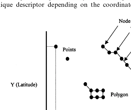
2.1.Vector GIS
‘arc’. Polygons are used in GIS to represent enclosed areas (Fig. 1). A polygon consists of a number of lines, but is distinguished by the characteristic that its starting and ending nodes are the same. For aquaculture applications, examples of polygons include a reservoir, a certain soil class, and a distinct type of land classification (e.g. a mangrove forest). Based on the coordinate system used, a vector GIS knows where the spatial feature (point, line or polygon) exists (i.e. its absolute location), and its relationship to other features (topology or relative location). As an example, a GIS would thus be aware that a reservoir supplying water to a fish farm is located north of the farm ponds.
After spatial features are represented in vector GIS, their associated properties can be specified in a separate database. As an example, properties of a soil polygon such as pH, bulk density, cation exchange capacity, and infiltration rate can be archived in a database. These properties are often referred to as ‘themes’, which can be presented in so called ‘thematic maps’. Vector GIS lend themselves well to the use of relational databases because once the spatial features are specified (once), any amount of related data can be associated with them. The term ‘coverage’ is used in the GIS literature to refer to the combination of a geographically referenced feature and its associated data. Thus, a ‘stream coverage’ would refer to the line in a vector GIS that represents its course, and the associated data such as flow rates, temperature, water quality characteristics, and withdrawal rates (and possibly spatial locations) for different uses.
2.2.Raster GIS
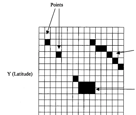
In a raster GIS, space is represented by a uniform grid, each cell of which is assigned a unique descriptor depending on the coordinate system used (Fig. 2).
Fig. 2. Representation of spatial features (points, lines and polygons) in a raster GIS (adapted from Thompson, 1998).
Thus, a cell in a grid that uses the latitude/longitude system would have a pair of coordinates. Numerical data pertaining to spatial features that are represented in the grid are assigned to the appropriate cell. Raster GIS can be conveniently thought of as being a spreadsheet, and one of the earliest GIS applications in aquaculture was essentially a spreadsheet-based system to assess carp culture possibilities in Pakistan (Ali et al., 1991).
imported into raster systems for further classification and display (Kapetsky and Nath, 1997). Similarly, raster GIS can be used to model effluents discharged by aquaculture operations into natural water bodies by applying appropriate equations to cells in the spatial grid (Perez-Martinez, 1997). Another advantage of raster GIS is that remote sensed data (which are usually stored in raster format) can often be directly imported into the software and immediately become available for use (Burrough, 1986).
2.3.Analytical scope, reporting and 6isualization
One of the powerful features of both vector and raster GIS packages is that statistical summaries of layers/coverages, model stages or outcomes can easily be obtained. Statistical data can include area, perimeter and other quantitative esti-mates, including reports of variance and comparison among images. A further powerful analytical tool that aids understanding of outcomes is visualization of outcomes through graphical representation in the form of 2D and 3D maps. For example, entire landscapes and watersheds can be viewed in three dimensions, which is very valuable in terms of evaluating spatial impacts of alternative deci-sions. Techniques have also been developed to integrate GIS with additional tools such as group support systems, that allow interactive scenario development and evaluation, and support communication among stakeholders via a local area network (LAN; Faber et al., 1997). There is also currently rapid development and deployment of Internet-enabled GIS tools, which allow a wider community of decision makers to have instant access to spatial data. All of these tools are constantly being added to GIS packages and are of great value if appropriately used. Presently available tools include Arc/Explorer and Internet Map Server (from ESRI, Inc) and MapXtreme (from MapInfo Corporation). Because GIS technology is evolving at a very rapid rate, we have chosen not to evaluate specific products. Information about GIS and related tools are, however, available from various Web sites including: http://www.utexas.edu/depts/grg/virtdept/resources/vendors/ ven-dors.htm and http://www.gislinx.com/. Guidelines for selecting GIS tools are available in: Burrough (1986), Meaden and Kapetsky (1991) and Burrough and McDonnell (1998).
3. GIS methodology
organization(s) and/or types of personnel, as well as according to the requirements of specific projects.
With regard to the first phase of any GIS project (basically a conceptualization and planning step that precedes actual implementation), our opinion is that it has traditionally been somewhat neglected both in the GIS literature as well as in practice. This is true despite the fact that it will likely determine the extent to which information generated by the use of GIS is used in real world decision making. The latter criterion, of course, is the ultimate yardstick by which success of spatial methods and technology will be measured over the long-term.
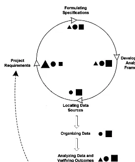
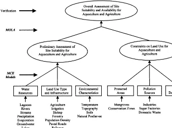
The phases involved in any GIS study (Fig. 3; described in detail below) occur iteratively in the sense that project personnel may often conduct a pilot-scale study
with available information, and then successively enhance and/or refine the analysis until a satisfactory end point is reached. Alternately, subsequent phases in the project cycle may result in new information that needs to be incorporated in the preceding phase(s). For example, it may become evident during the development of the analytical framework that requirements documented during the first iteration of the project cycle (Fig. 3) may need to be revised.
Recognizing the iterative nature of a GIS study allows the entire project team to develop an improved understanding of the issue on hand, and how spatial methods and technology can be best be used to address it. Once project personnel explicitly recognize that GIS work is iterative in nature and begin to document what is learnt during each phase, it becomes easier to track how user requirements are explicitly addressed during implementation (often referred to as traceability in the software literature; Ambler, 1998), and to deliver timely as well as meaningful project updates (e.g. GIS outputs and reports).
3.1.Identifying project requirements
The process of identifying requirements for a GIS is essentially a multiple stakeholder decision-making situation. This is because such work is invariably executed by a group of subject matter experts and analysts, and because results of the analyses are potentially useful to a range of decision-makers. Individuals in these three broad groups of stakeholders are likely to have different perspectives and expectations with regard to the capabilities and limitations of GIS. It is important that these perspectives and expectations are allowed to surface during the early stages of GIS work so that an enabling environment can be created within which decision support needs of end users are discussed and project goals formulated.
Once project personnel, particularly end users, have had an opportunity to present their spatial decision support needs, discussions can begin to examine how GIS tools can address these needs, and clarify the limitations of such tools (e.g. spatial data availability and quality, software/hardware resources that may be needed, cost and time constraints, etc.). At this stage, it is usually not necessary or even productive to invest an inordinate amount of time in discussing these issues. Instead, the intent is to develop common understanding about decision support needs, specify project goals, clarify GIS functionality and develop a listing of general requirements. More importantly, such discussions can facilitate the develop-ment of a creative and productive project team, wherein each participant has an opportunity to identify their own roles and responsibilities, and those of their partners.
The above observations are consistent with the work by Campbell (1994) (see also Campbell and Masser, 1995), who suggests that the following factors are important in successful GIS implementation and its subsequent use in decision-making:
an information management strategy in which the needs of users are clarified,
identification of simple applications that generate information fundamental to
the work of potential users;
implementation that is user-directed, and which has the commitment and
partic-ipation of staff throughout the organization(s) involved; and
the ability for the organization(s) to create sufficient stability or to be able to
cope with change, both in terms of evolving specifications and rapidly changing technology.
In our own experience, there has been a tendency among some of the technical assistance organizations with which we collaborate to invest a considerable amount of time, effort and financial resources in developing GIS capabilities and acquiring expensive spatial datasets. However, it is often the case that this investment is made without a clear understanding about what they wish to accomplish with such capabilities, and the stakeholder groups (both within and outside the organization) whose decision support needs they are attempting to fulfil. More often than not, GIS capabilities of such organizations are primarily used as a tool for generating and displaying maps. The current state of spatial methods and technology, on the other hand, clearly indicates that GIS capabilities go beyond data management and visualization alone.
For instance, process-based models and GIS (especially raster systems) are very complementary tools in that the former can be used to generate new output layers from multiple base maps already in GIS format. The derived layers often contain information that is more useful to decision-makers. Moreover, it is now possible to directly integrate within GIS models that have distributed (i.e. spatially explicit) parameters, and to seamlessly run alternate scenarios within a single software package. Prior to the availability of such techniques, it was necessary to execute multiple model runs outside of a GIS environment, and to import the output into GIS for visualization. Such indirect coupling often requires additional time and technical expertise to handle model management and data transfer requirements, besides limiting the range of scenarios that end users may wish to analyze. Direct integration of models within GIS, however, has the potential to enable such users in the aquaculture domain to explore alternate scenarios in a truly interactive way, simultaneously reducing the need for the continued presence of analysts or at least using their expertise in a manner that is more cost effective. The trend towards interactive GIS use is already evident in both in the business world and in some natural resource management domains such as conservation efforts.
specific techniques to manage the process are not unique to GIS applications, but are increasingly recognized within a number of domains including organizational development (Adams, 1986; Senge, 1990), concurrent engineering design (Voland, 1992), and information technology (Ambler, 1998).
3.2.Formulating specifications
The goals and requirements of the project articulated in the first phase above are by necessity of a general nature. This is largely because it is rarely productive to embark upon an exercise to specify project components without a broad under-standing of decision support needs. Furthermore, if team members begin to focus too much on project specifics early on in the overall process, they run the risk of not being able to adequately accommodate additional needs of end users (given that such needs usually tend to evolve over time), and of already confining themselves to a certain mindset about implementation strategies.
However, once an overall understanding of project requirements has been developed among team members, it is helpful to develop a listing of more functional specifications corresponding to each of the requirements that have been identified. For instance, if the project requires that the final GIS be interactive (implying that the end user can explore alternate scenarios on their own), one or more of the following are representative of possible functional specifications:
capability of generating and editing different thematic maps;
features for querying attributes in spatial databases;
support for adding new themes and/or updating current information in the GIS over time;
enabling application of the analytical approach to different geographical regions; and
capability to modify existing models and/or link new models to the GIS. The process of identifying functional specifications involves an in-depth analysis of each of the project requirements. In practice, it is usually beneficial for the subject matter experts and GIS analysts to first formulate project specifications jointly, and to then share these with the end users. This approach tends to result in time (and therefore cost) savings. Moreover, the need for communicating (poten-tially) difficult technical concepts is minimized because end users are likely to be more interested in the actual specifications, rather than in the process by which they were determined.
same author, it is safe to assume that no project can ever be fully specified (particularly during the initial phases of development) and a judicious end point for this phase must be identified to ensure that timely progress towards the overall goals is maintained. It is also often the case that when functional specifications are identified, project personnel may identify new requirements, which need to be appropriately documented with existing information from the first phase of the overall project (i.e. identifying project requirements; Fig. 3).
3.3.De6eloping the analytical framework
The previous two phases deal primarily with aspects of what is to be accom-plished (i.e. project needs). Development of the analytical framework for a GIS project, on the other hand, addresses issues of how these needs will be addressed. This phase largely involves subject matter specialists and GIS analysts (Fig. 3). However, consultations with end users are recommended to ensure that the project will indeed address their needs, to accommodate new needs that may arise, and to foster an improved understanding of analytical methods that may be used. An understanding of the methods used, as well as their limitations, is critical in terms of appropriate application of GIS outcomes for decision support.
Several methods have been used, either singly or in combination, by GIS practitioners to integrate spatial information into a useful format for analysis and decision making. The following represent analytical methods that have already been used in aquaculture GIS or have potential for use in the future. Their inclusion here is intended to provide readers with an overview of the range of analytical methods that may come up for discussion during this phase of a GIS project.
3.3.1. Arithmetic operators
A large number of arithmetic operators can be used in GIS (Burrough, 1986). For instance, a useful precursor is the scalar operation in which a constant term is to be applied to spatial data (e.g. to estimate the potential annual consumption of fish in a region, the population size of towns can be multiplied by a constant representing the annual fish consumption per capita). Another example would be the subtraction of monthly evapotranspiration and seepage layers from a precipita-tion layer to estimate mean monthly water requirements for ponds (Aguilar-Man-jarrez and Nath, 1998).
3.3.2. Classification
sensible decision making at a later stage (Burrough, 1986; Aguilar-Manjarrez, 1996; Ross, 1998).
Aguilar-Manjarrez (1996) provides an exhaustive review of five methods that have been explored to classify data on land types for various uses:
1. The FAO land evaluation methodology which assesses land suitability in terms of an attribute set corresponding to different activities.
2. The limitation method in which each land characteristic is evaluated on a relative scale of limitations.
3. The parametric method in which limitation levels for each characteristic are rated on a scale of 0 to 1, from which a land index (%) is calculated as the product of the individual rating values of all characteristics.
4. The Boolean method which assumes that all questions related to land use suitability can be answered in a binary fashion, and that all important changes occur at a defined class boundary.
5. The fuzzy set method in which an explicit weight is used to assess the impact of each land characteristic. Fuzzy techniques are then used to combine the evalua-tion of each land characteristic into a final suitability index. Apart from a dominant suitability class, the fuzzy set method equally provides information on the extent to which a certain land unit belongs to each of the suitability classes discerned.
For GIS applications, any of the above methods can be used to classify source data into a four- or five-point scale of suitability (with one being the least suitable). However, the choice among classification methods is dependent on the type of data and intended uses of the output information. Classification allows normalization of all data layers, an essential pre-requisite for further modeling. An example is the grouping of soil data into four classes based on a number of properties important for pond construction (Kapetsky and Nath, 1997).
3.3.3. Simple o6erlay
3.3.4. Weighted o6erlay
In decision making, it is usually the case that different attributes under consider-ation do not have the same level of importance. This calls for a weighted overlay approach, in which each layer is assigned a weight that is proportional to its importance. To accomplish this, each source layer is first reclassified onto a common scale and then multiplied by a weighting factor. The resulting values are used in further overlay operations to obtain an outcome (applying Boolean constraints in the final stage if needed).
The derivation of weightings for source attributes is often assumed to be an objective scientific matter. However, it is clear from a range of studies that even expert opinions on ranking of attributes may differ substantially. Aguilar-Manjar-rez (1996) showed that, from a list of attributes, a group of experts with similar backgrounds generally agree upon which are the most relevant to use for any given decision process. However, the ranking assigned to the attributes by these experts can differ. In general, Aguilar-Manjarrez (1996) showed that from a list of ten selected attributes, different experts would be in agreement on the priority of the first three to four and the last three. However, attributes with mid-level priority are often dealt with quite differently. Moreover, subject matter experts with different backgrounds (e.g. aquaculturist, coastal zone planner, conservationist, etc.) bring differing agendas to the same problem, resulting in a range of outcomes. At worst, it is clear that without guidance, a range of prioritizations can be obtained which are cumulatively meaningless. GIS analysts therefore need to ensure that weightings applied personally are as objective as possible and that where expert group input is used, the basis for this input is fully explained and carefully analyzed before its use for decision making. Summary tables that transparently document factors used in the evaluation and the weights assigned to them by different experts are a useful aid in this regard (Aguilar-Manjarrez, 1996; Aguilar-Manjarrez and Nath, 1998).
assign weights to the factors. In general, it is unlikely that technical methods such as AHP or other multi-criteria decision making tools (see review by Merkhofer, 1998) can be a complete replacement to a well-facilitated exercise in which stakeholders (i.e. subject matter specialists, GIS analysts and end users in the current context) are encouraged to seek consensus on the relative importance of attributes for use in GIS. Instead, such tools should be viewed as providing additional support to the consensus building process.
3.3.5. Neighborhood analysis
A key function provided by GIS, and one which cannot be easily addressed by the use of any other decision support tool, is its capability to allow evaluation of the characteristics of an area that surrounds a specific location, which is referred to as neighborhood analysis. GIS software provides a range of neighborhood func-tions including point interpolation techniques in which unknown values are esti-mated from known values of neighboring locations. These techniques are typically used to convert point coverages into grids or to generate elevation data either in triangular irregular network (TIN) format for vector GIS or as a digital elevation model (DEM) for raster GIS. DEMs have not as yet found widespread use in aquaculture, but are often at the heart of environmental GIS that are targeted towards analyses of entire landscapes. For instance, the DEM for a watershed of interest is a key layer in many spatially explicit hydrological models. In the future, such tools are likely to find applications in aquaculture from the perspectives of assessing water availability and modeling environmental impacts of existing and/or proposed aquaculture operations. A common type of neighborhood operation is buffering, which allows the creation of distance buffers (or buffer zones) around selected features. An example where this operation may be useful in aquaculture is when there is a need to determine how many streams are available (or to be avoided) within a specified distance of a proposed facility.
3.3.6. Connecti6ity analysis
This type of analysis is characterized by an accumulation of values over the area that is being traversed. Support for connectivity analysis in commercially available GIS software is not as standardized in comparison to the operators described above. Network analysis is one type of connectivity operation, which is character-ized by the use of feature networks such as hydrographic hierarchies (i.e. stream networks) and transportation networks. As an example of the use of network analysis in aquaculture, Kapetsky and Nath (1997) estimated the shortest trans-portation path from a given site to the nearest market.
3.3.7. Hierarchical models
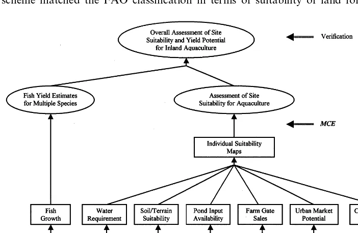
In practice, comprehensive representation of the real world in a GIS often involves the use of a large number of source variables, which when processed into GIS using one or more of the analytical methods described above, may result in considerable complexity. Experience suggests that when the number of layers exceeds about 10, MCE becomes difficult, even to the experienced modeler. Such situations warrant the development of a hierarchical modeling scheme.
In this approach, naturally grouped variables are first considered together to produce ‘sub-model’ outcomes such as water needs, soil suitability, input availabil-ity, farm gate sales, and markets (Kapetsky and Nath, 1997). It is often the case that a source variable or processed layer will be used in more than one sub-model and that the layer may need to be transformed depending on the intended purpose. Each of these sub-models may, in turn, be derived from lower-level models which pre-process variable data into useful factors. Another example from aquaculture is the estimation of wave height from wind velocity and fetch (Ross et al., 1993).
It is, of course, not necessary to embed all of the models and/or sub-models within a single system per se. This is because commercial GIS can export and import information quite seamlessly with external modules. For instance, growth estimates derived from an external bioenergetic model (linked to spatial weather and water temperature datasets) have been used to predict fish yields in continental-scale GIS (Kapetsky and Nath, 1997; Aguilar-Manjarrez and Nath, 1998). In a different context, external rule-based systems are being used in conjunction with GIS to generate future agricultural land use patterns for assessing policy alterna-tives in the Pacific Northwest region of the United States (Bolte, unpublished information).
3.3.8. Multi-objecti6e land allocation
3.4.Identifying data sources
Once the analytical framework has been developed, it is necessary to identify data sources to be used in the project. This phase is largely restricted to GIS analysts (Fig. 3), although subject matter specialists often provide helpful advice (e.g. identifying non-spatial datasets). Information for spatial decision-making and analysis is varied, and will usually consist of data describing the biophysical, economic, social and infrastructural environments. These data can come from a variety of sources ranging from primary data gathered in the field or satellite scenes to all forms of secondary data, including textual databases and reports.
It is generally both costly and time consuming to collect field (primary) data first hand. Therefore, all GIS practitioners attempt to locate the data they need from existing secondary sources, either in paper or digital form. The initial consideration is identifying what data are needed for the overall analysis. This is followed by attempts to source the data, and to assess their age, scale, quality and relative cost. Different data types are often developed in different geographic coordinate systems, and must be re-projected onto a common coordinate system. Other common issues are ensuring that features common across multiple layers are spatially coincident, and understanding the resolution, constraints and uncertainty associated with the data. For these reasons, data collection and preprocessing are typically the most expensive and time-consuming component of an analysis.
Digital database availability is increasing at a rapid rate throughout the world. These databases contain information ranging from natural resources (e.g. maps of soils, water resources and temperature distributions), to population census and cadastral (i.e. property ownership and associated boundaries) data. In many cases, such data may only be available in hard copy reports, although information is also available on CD-ROMs, from which databases for GIS use can be extracted.
A further source of data is the WWW, from which a wide range of mapped and other spatial data can be found by carefully executed searches. Spatial information at low resolution can often be obtained in this way, good examples being the Global 30 arc second elevation (http://edcwww.cr.usgs.gov/landdaac/gtopo30/
Thematic data can be in the form of a choropleth (areas of equal value separated by boundaries), isopleth (lines which connect points of equal value) or point maps (Burrough, 1986), all of which are often valuable, a good example in terms of aquaculture being the hydrographic chart. The more common topographic map frequently contains many thematic data (including elevations, water bodies, roads, cities, and woodlands) which are of value to the GIS analyst. These themes can be extracted at the stage of digitization, and established as separate layers in the spatial database.
3.5.Organizing and manipulating data
After datasets have been collected, it is necessary to organize and manipulate them for use in the target GIS. This phase is also largely restricted to GIS analysts (Fig. 3), although depending on the type of application, occasional interaction with subject matter specialists may be warranted. Some of the key activities that occur in this phase include verification of data quality, data consolidation and reformat-ting, creation of proxy data and database construction. Proxy data refer to information that is derived from another data source, for which established relationships may exist. Examples include estimation of water temperature from air temperature (Kapetsky, 1994), extraction of semi-quantitative texture from FAO soil distribution maps (Kapetsky and Nath, 1997) or calculation of maximum wave heights from wind speed and fetch (Ross et al., 1993).
In terms of verification of data quality, the reliability of thematic maps world-wide is variable, as is the currency of their content. These aspects must be considered where critical decisions are based upon such material. Although digital maps are often quite up to date, the spatial accuracy of some printed material can be suspect. Critical assessment and verification of source data quality is very important. The value of such verification for all input data cannot be over-stressed, before digitizing as well as after the fact. It is usually the case that at least some of the layers required in a GIS database will not be of a high enough standard, and verification on paper may very well need to become verification by survey, where warranted. A detailed overview of technical methods to address data quality issues is available in Burrough (1986).
Certain data sources such as satellite data are already in digital form, but all others may require some work in order to consolidate them for spatial analysis. Satellite images provide a rich source of data in a form suitable for use in a spatial database. The information collected by the scanners on LANDSAT and SPOT are aimed specifically at natural resource work and the source data can be reprocessed in a variety of ways to reveal details of the environment that may not be apparent in the raw state.
land uses, often in some detail. A number of widely used vegetation indices, such as normalized difference vegetation index (NDVI), can also be calculated and the resultant thematic data extracted for immediate use in GIS. A potential example in aquaculture would be the development of an algal bloom index to assess the risk of fish kills due to dissolved oxygen depletion in pond systems. The digital nature of the product means that the data are easy to incorporate and their relative costs low compared to primary data collection surveys. Remotely sensed images are therefore a common starting point for GIS work.
Reformatting of data for use in a particular GIS may also include classification of the information (as discussed in the preceding section on analytical methods) and conversion of available data from vector to raster format (or vice versa). Finally, spatial data are often available at different resolutions, and it is necessary to convert the datasets to the desired scale for the analysis to ensure appropriate data processing. This may very well involve seeking expert opinion on the validity of reconciling scale differences.
Database construction is another set of activities that is typically undertaken in this phase. Designing an appropriate database is important both in terms of ensuring that the information can be readily accessed for the target application, and is available for re-use at a later time. It has been the case in the past that spatial data were usually stored in formats suited to the type of GIS software being used. This often resulted in spatial databases that were not relatively easy to extract either for use in other types of applications or software. However, many organizations are taking advantage of recent advances both in GIS and database technology by storing both raw and processed information in relational databases. Such data can seamlessly be imported for use in stand-alone GIS applications, but are in principle available for alternate uses (e.g. data publishing across the WWW).
3.6.Analyzing data and 6erifying outcomes
This phase represents the culmination of effort that has been expended, particu-larly on the part of GIS analysts, to develop the analytical framework, locate data sources and organize data for the analysis. As can be expected, the GIS analysts play the most important role in this phase but are likely to interact with subject matter specialists and end users in terms of verifying preliminary results (Fig. 3). Activities that may be encountered in this phase include executing analytical methods (i.e. overlays, model runs and/or other querying knowledge based systems, etc.), importing and exporting data as needed (e.g. intermediate GIS outputs which are required by other components within the overall analytical framework), compu-tation of relevant statistics (e.g. means, standard deviations, ranges, classes, etc.), generation of output information (e.g. maps, tables, graphs, and reports), and verification of outcomes.
Fieldwork as part of a verification exercise is frequently referred to as ground-truthing. The general approach to such work is similar to any field survey, and standard techniques for survey, and environmental measurements can be used. The main difference is in the sampling plan and a verification exercise will typically be based on a series of sample points designed to cover the area. Such coverages would normally be well distributed over the ground or water surface, but are often more efficient if a random stratified sampling pattern is used. This allows effort to be concentrated on ensuring that differences between different features in the land-scape are assessed, rather than using a simple randomized pattern, which may repeatedly cover a large uniform area.
Global positioning systems (GPS) have greatly aided the spatial accuracy of ground-truthing and field verification, in most cases removing the need to use surveying techniques completely. These systems provide three-dimensional position locations from satellites to within about 100 m under normal operation, although actual accuracy is frequently as good as 20 m or even less. By operating in differential mode, two GPS units can give real-time locations accurate to less than a meter and with post-processing to within a few millimeters (Aguilar-Manjarrez, 1996). The value of these systems has been rapidly recognized by GIS practitioners. Some GIS data acquisition systems will accept direct input from GPS so that the location can be displayed over a real satellite image of the study area.
Apart verifying data and outcomes of models, field verification can provide feedback into the analytical process itself by allowing the GIS analysts and subject matter specialists to understand, quantify and document errors of the assumptions used. Such documentation should be an integral part of the overall project report.
3.7.E6aluating outputs
Little work has apparently been done in the area of indicator monitoring by personnel involved in aquaculture GIS, perhaps because many of the efforts to date have been undertaken primarily as academic exercises. In other contexts where GIS have been developed by technical assistance organizations, it would appear that an implicit assumption by the implementing personnel is that if the information is produced, the target audience of decision makers would actually use it. However, because end users have often not been consulted in aquaculture GIS projects (as previously indicated), this assumption is somewhat questionable. Clearly, there is need for typical end users, subject matter specialists and spatial analysts to collaborate more actively in the development and application of GIS for aquaculture.
4. Case studies in aquaculture
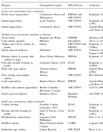
The use of GIS in aquaculture, together with selected cases, has previously been documented (Meaden and Kapetsky, 1991; Kapetsky and Travaglia, 1995; Aguilar-Manjarrez, 1996; Ross, 1998). In this section, we build on the foundation that has been set forth by the above authors, specifically examining selected cases (in some detail) from the perspective of their applications for spatial decision support in aquaculture. A more comprehensive listing of GIS applications for aquaculture is presented in Table 1 (see Meaden and Kapetsky, 1991 and Aguilar-Manjarrez, 1996 for other examples).
The selected cases represent a broad sampling across geographic scales ranging from local areas (i.e. a small bay), to sub-national regions (i.e. individual states/
provinces), to national and continental expanses. They also vary with regard to the degree to which GIS outcomes have been used for practical decision making. Further, the case studies demonstrate the large extent of GIS applications that are possible in aquaculture including: site selection for targeted species, environmental impact assessment, conflicts and trade-offs among alternate uses of natural re-sources, and consideration of the potential for aquaculture from the perspectives of technical assistance and alleviation of food security. The cases also vary signifi-cantly with regard to complexity of the analytical methods used (i.e. ranging from simple overlays to weighted combinations to use of relatively sophisticated models). Finally, the case studies are indicative of issues associated with data procurement and manipulation, and the diversity of GIS packages that are available. Each of the case studies is presented in the following format:
source of the work;
objectives;
target decision support audience;
geographic area and scale of analysis; analytical methods and results; and
comments (e.g. limitations of the approaches used, possible enhancements, and
Table 1
GIS applications in aquaculture according to the kind of assessment and scale of study (adapted and updated from Kapetsky and Travaglia, 1995)
Author(s) GIS Software
Purpose Geographical region
Large area assessments(low resolution)
Warm water aquaculture Continental Africa and ERDAS and Kapetsky (1994) Madagascar ARC/INFO
Inland aquaculture Latin America ARC/INFO Kapetsky and Nath (1997)
Inland aquaculture Continental Africa ARC/INFO Aguilar-Manjarrez and Nath (1998) Medium area assessments(medium resolution)
Meaden (1987)
Fish and crayfish farming in ELAS Kapetsky et al. (1990b) ponds
IDRISI
Pond and cage culture Tabasco (State), Aguilar-Manjarrez
Mexico (1992)
ARC/INFO
Fish, shrimp and mollusc Tunisia Ben Mustafa (1994) culture Small area assessments(high resolution)
ELAS Kapetsky et al. Franklin County,
Catfish farming
(1988) Louisiana, USA
Shrimp and fish farming in Gulf of Nicoya, Costa ELAS Kapetsky et al. Rica
Camas Bruaich Ross et al. (1993) Salmonid cage culture
Ruaidhe Bay, Scotland for-the-PC
Shellfish culture Sepetiba Bay, Brazil IDRISI Scott et al. (1998) ArcView Arnold et al. (2000) Indian River Lagoon,
Shellfish culture
4.1.Site selection for salmonid aquaculture, Scotland (source:Ross et al., 1993)
4.1.1. Objecti6es
The primary objective of this work was to examine GIS as a tool for assessing the potential of salmonid cage aquaculture in a small bay. A secondary objective was to develop a general methodology for spatial analysis of coastal cage aquaculture potential.
4.1.2. Target decision support audience
A specific audience for this work was not identified by the authors perhaps because the work was primarily a research effort to investigate the feasibility of using GIS for assessing cage culture potential at a local scale (i.e. fine resolution). Nevertheless, the outcomes of the study and the GIS per se would certainly be of interest to governmental agencies responsible for promoting and/or monitoring aquaculture development in the bay, and to individual investors wishing to identify suitable sites for cage culture.
4.1.3. Geographic area and scale of analysis
The study area comprised the Camas Bruaich Ruaidhe Bay located along the West Coast of Scotland. The bay is only 19.8 ha in size. Two scales of resolution (25×25 m, and 10×10 m) were pursued in the study, of which the coarser scale was found to be unsatisfactory for processing of most data. As noted by the authors, however, the issue of scale is typically a trade-off between data needs/
availability and objectives of the GIS work. In this case, the finer resolution was more appropriate.
4.1.4. Analytical methods and results
This study used a successive screening process for different criteria identified to be of importance in evaluating aquaculture sites, and application of simple overlay techniques within a very low cost raster GIS (OSU-MAP for the PC). The criteria included depth, current velocity, salinity, dissolved oxygen, and temperature (con-sidered to be key factors in salmonid cage culture), as well as other factors (i.e. local infrastructure, topography and exposure). With the exception of local infrastructure (judged to be quite suitable for aquaculture based on a qualitative assessment of accessibility to markets, and availability of labor, services and supplies), all of the other criteria were analyzed spatially for the entire bay.
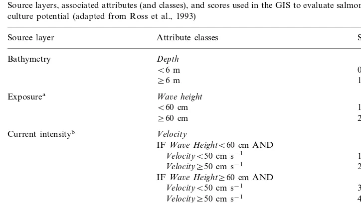
More specifically, the GIS analysis involved overlaying the base topographic map with each of the above layers to obtain independent maps depicting their spatial characteristics. Following this step, a sequential procedure (in which suitability scores were assigned to each attribute; Table 2) was used in successive overlays to arrive at a final assessment of salmonid cage culture potential. In terms of criteria used for each attribute, depth and salinity information (Table 2) essentially serve as constraints in that a score of zero implies that the site is not suitable from the perspective of adequate depth to support cage culture or salinity fluctuations exceeding the tolerance of the target species. The combination of exposure and current intensity, on the other hand, allow alternative sites to be classified into a wider range of suitability categories (1=Most suitable and 4=Least suitable). Example output from such a GIS likely to be of most interest to the target audience of decision-makers would be the final map in which the results of a set of spatial operations similar to those described above (and in Table 2) are added to the base topographical layer so as to show the potential for salmonid cage culture.
4.1.5. Comments
According to Ross et al. (1993), only about 6% of the areal expanse of the bay would be suitable for cage culture. Their analysis essentially corresponded to a
Table 2
Source layers, associated attributes (and classes), and scores used in the GIS to evaluate salmonid cage culture potential (adapted from Ross et al., 1993)
Scores Source layer Attribute classes
Bathymetry Depth
0
B6 m
]6 m 1
Exposurea Wa6e height
B60 cm 1
]60 cm 2
Current intensityb Velocity
IFWa6e HeightB60 cm AND
VelocityB50 cm s−1 1
2 Velocity]50 cm s−1
IFWa6e Height]60 cm AND
VelocityB50 cm s−1 3
Velocity]50 cm s−1 4
Salinity6ariation Salinityc
B8 ppt 1
]8 ppt 0
aData layer added to the output resulting from the bathymetric scoring, and exposure scoring criteria
applied.
bData layer added to the output from the previous set of operations, and current velocity criteria
applied.
situation of ‘worst-case modelling’ in that wave heights, for instance, were com-puted based on the longest recorded fetches and highest wind speed combina-tions. In other words, the possibility exists that a larger area of the bay would be suitable for cage culture. Apart from the data used in GIS analyses of this nature, the ‘sequence’ in which spatial operators are used will influence the output (Burrough, 1986; Ross et al., 1993). Thus, if the original decision se-quence (i.e. depth, exposure, current intensity, and salinity) is changed, the ensuing output will be different because of Boolean algebraic operations. It is therefore important that analysts involved with GIS work closely with subject matter experts to establish the priority of different criteria, which in turn estab-lishes the sequence of spatial operations.
This case study is indicative of the potential advantages associated with GIS use for site selection over manual evaluation — the authors in fact made a comparison of time and resource requirements between GIS use and physical assessment by aquaculturists. They concluded that in terms of time, the GIS was more efficient. However, it was more costly to conduct the GIS work, as opposed to a manual assessment — on the other hand, these costs are expected to decline substantially as the tools and techniques are used for addi-tional projects. Moreover, if the GIS were to be refined for use in routine monitoring (e.g. pollution assessment of the bay due to cage culture), its benefits as a management tool would clearly outweigh the investments over the long term. Finally, Ross et al. (1993) proposed a set of guidelines whereby a generic GIS logic sequence could be used for site selection in coastal waters. The guidelines involve screening out locations where depths are unsuitable, grading areas that do have adequate depth on the basis of wave heights (simultaneously addressing engineering specifications for the possible types of cages), grading the resulting areas according to the range of current velocities, and finally examining water quality parameters in terms of their suitability for the target culture species (in the geographic location where their work was conducted, oxygen and temperature were not limiting factors but may very well be in other places).
4.2.Assessment of land suitability for aquaculture and agriculture in Sinaloa State,
Mexico(sources: Aguilar-Manjarrez and Ross, 1995; Aguilar-Manjarrez, 1996)
4.2.1. Objecti6es
The main objective of this work was to develop a detailed GIS that could serve as an analytical and predictive tool to guide (shrimp) aquaculture development at a state-level in Mexico. The GIS was intended to provide planners and managers with a tool to assess land suitability for aquaculture and agriculture in the state of Sinaloa, and to provide guidance for exploring the consequence of land use decisions before they are committed to action. Aguilar-Manjarrez (1996) also extended the GIS to allow evaluation of shrimp aquaculture opportunities at an individual ‘site’ (the Huizache Caimanero Lagoon in Sinaloa). This work is not discussed here due to space constraints.
4.2.2. Target decision support audience
The GIS developed by the authors (as well as outcomes generated) would be of interest to governmental agencies responsible for promoting and/or monitoring shrimp aquaculture development in the Sinaloa State of Mexico. More likely than not, information generated would be useful for decision making at the state, regional and national levels. Investors keen on large-scale operations would also be interested in identifying opportunities for shrimp culture where the potential for production is high, and conflicts with agricultural use of the land likely to be limited.
4.2.3. Geographic area and scale of analysis
The study area comprised the zone between 22° 12%– 27° 13%N and 105° 19%– 109° 33% W ensuring coverage of the entire state of Sinaloa (located along Mexico’s
northwest coastline), areas of neighboring states (Sonora, Chihuahua, Durango, and Nayarit) and the Gulf of California. The authors report the area of the Sinaloa state to be roughly 58 480 km2. Spatial analysis was conducted at a resolution of
250 m.
4.2.4. Analytical methods and results
Fig. 4. A hierarchical modeling scheme with MCE and MOLA to evaluate suitability of locations for aquaculture and agriculture and resolve associated conflicts, in the Sinaloa state of Mexico (adapted from Aguilar-Manjarrez and Ross, 1995).
After suitability classes were assigned, the factors were weighted by the use of the AHP technique. This was followed by generation of factor maps, which in turn were multiplied by the various constraints to mask out unsuitable areas. The process of classifying factors, their weighting, generation of maps, and application of con-straints involved the use of an automated MCE procedure in IDRISI.
The final step in the analysis was to apply the MOLA technique in order to maximize the land allocation area for aquaculture and agriculture. The rationale behind the use of this technique was that aquaculture and agriculture are often in conflict because they require similar types of infrastructure, share a number of common biophysical requirements, and have parallel economic and social impacts. Use of the MOLA technique requires assignment of weights for each of the alternative activities under consideration — for this study, equal weights were assigned for aquaculture and agriculture. Outcomes of the various steps listed above (see also Fig. 4) included suitability maps for both aquaculture and agriculture, and a single map depicting areas found by the MOLA technique to be most suitable for these two land use activities (Fig. 5).
The GIS analysis and predictions in this study were entirely dependent on a variety of information sources (which themselves are likely to have some level of inaccuracy) and even different scales. Hence, it was considered to be of paramount importance to carry out field verification. Moreover, it was also considered to be very important to locate other data (e.g. pollution sources or other relevant information) which were either not identified or required updating during the creation of the original database. This involved the use of GPS (see Aguilar-Manjarrez, 1996 for full details) to locate points on the ground, and comparison of GIS output to results of a manual survey conducted by two Mexican consultancy firms. The verification exercise suggested that although the areal expanses suitable for aquaculture were comparable between the GIS and manual survey results (roughly 2090 km2
or about 3.5% of the area of Sinaloa), suitable locations that were identified differed among the two methods. This was presumably because of differences in the logic and analytical techniques used. However, it would appear that outcomes from the GIS were more indicative of the true potential for aquaculture because of the range of criteria considered and their integration into suitability models. Moreover, the GIS was able to identify and resolve areas of potential conflict between agriculture and aquaculture. In principle, such information can be helpful to decision makers in terms of exploring alternative land use practices ‘prior’ to committing them to the landscape.
4.2.5. Comments
In terms of routine use for decision making, some of the drawbacks of this GIS include limitations of the IDRISI software from the perspective of allowing users to truly interact with the decision models (e.g. easily formulating and executing ‘what-if’ scenarios) and generating reports of analyses undertaken. We discuss these issues in more depth within the case study from British Columbia (see below).
This case study could be even further enhanced by the use of analytical methods that have since been developed and applied to aquaculture. For example, in addition to the criteria used, comprehensive analysis of site suitability should include consideration of the potential impacts of land-based aquaculture on surface and ground water resources (e.g. by the use of more recent techniques to model waste dispersion from aquaculture farms as in Perez-Martinez, 1997). The GIS would also likely benefit from integration of its output with economic analysis and marketing tools which can allow a more comprehensive examination of the costs as well as benefits associated with aquaculture and agriculture. Finally, as noted by the authors, the GIS should also be expanded to address land use options besides aquaculture and agriculture (e.g. urban development, forestry, and livestock rearing) if it is to serve as a comprehensive tool for sustainable resource use planning in the state of Sinaloa.
4.3.Shellfish and finfish aquaculture management in British Columbia, Canada
(sources: Carswell, 1998; EAO, 1998; LUCO, 1998)
4.3.1. Objecti6es
The primary objective of the work represented by this case study was to develop a fully integrated information system (British Columbia Aquaculture System (BCAS); Carswell, 1998), within which GIS tools play a key role, to provide guidance for assessment of site capability for shellfish and finfish aquaculture. Although BCAS also includes inventories of marine plants (e.g. Nori, kelp) which can be accessed for use by personnel interested in farming them, we do not address this aspect in the case study.
4.3.2. Target decision support audience
BCAS represents one effort within an overall set of governmental initiatives in Canada to compile information required for land use planning, and related resource management. Within the province of British Columbia, these initiatives include efforts by local governments, federal and provincial governmental agencies, and the First Nations. Development and management of BCAS is an activity of the Ministry of Agriculture, Fisheries and Food (MAFF). At the time it was conceived, BCAS was intended to generate marine aquaculture information that would be of use for the development of policies at the provincial level (e.g. as part of land and resource management plans). Decision-makers at this level continue to be a target
Fig. 5. GIS maps indicating suitability classes of land areas for agriculture and aquaculture in the Sinaloa of Mexico (Source: Aguilar-Manjarrez and Ross, 1995).
audience, but use of BCAS has evolved in a hierarchical manner to include local governments in British Columbia as well as individual farmers (or entrepreneurs). For instance, decision-makers in various governmental positions routinely consult with GIS analysts not only to evaluate aquaculture potential, but to combine such analyses with information about unemployment rates and per capita income in order to set policies that potentially facilitate aquaculture development in disadvantaged zones (Carswell, MAFF, personal communication). Carswell also indicates that BCAS is being used by private consultants to advise farmers with regard to identifying suitable sites for shellfish aquaculture. However, because of a current moratorium on further development of finfish aquaculture, this module is not being as extensively used at the current time.
4.3.3. Geographic area and scale of analysis
BCAS includes marine resource inventories for the province of British Columbia, which has a coastline of about 29 489 km. Spatial assessment of sites for both shellfish and finfish operations are typically conducted at a scale of 1:40 000 (LUCO, 1998).
4.3.4. Analytical methods and results
BCAS includes a range of inventories (e.g. all marine plants, existing and proposed sites for aquaculture, etc) compiled by the aquaculture and commercial fisheries branch of MAFF. In addition, the system interfaces with digital data on a range of spatial biophysical and land use variables, which have been compiled by British Columbia’s Land Use and Coordination Office (LUCO). The biophysical variables are used within BCAS to estimate capability indices of sites to support shellfish and/or finfish aquaculture. The digital databases in which the biophysical variables are archived (and updated) are also used for a range of other applications (e.g. analysis of oil spillage impacts and associated remedial measures, ecological classification of British Columbia’s marine resources, etc.), and represent an excellent example of how spatial databases can be effectively employed by multiple organizations for sustain-able natural resource management.
In terms of the technology used, BCAS is a Windows-based, menu driven GIS/database application that automates analysis, integration and display of site capability indices for shellfish and finfish aquaculture. The system uses Borland’s Delphi programming language to link the Borland Database Engine and Report Smith with the ArcView GIS software. The database engine is used to access and manipulate data, and to calculate site capability indices on demand. The latter functionality is accomplished by accessing specific modules that have been separately developed to assess the potential for shellfish and finfish aquaculture (see below). The Report Smith tool allows creation of standard tables following any user-specified analyses. Finally, the ArcView component displays the site capability for the chosen aquaculture species, again in a standardized (mapping) format.
4.3.4.1.Site capability index(SCI)for shellfish. The shellfish module in BCAS uses
evaluate the capability of a potential site to support the culture of Pacific Oyster, Japanese Scallop and Manila Clam. The criteria are organized into the following subgroups (Cross and Kingzett, 1992):
direct impact on growth: water temperature, chlorophyll A (a measure of food availability), fetch, and exposure;
direct impact on survival: suspended sediments, tidal flow, fouling/disease/ preda-tors, substrate and beach slope (the latter two variables are used only for bottom culture); and
indirect impact of water chemistry on growth/survival: salinity, dissolved oxygen, and pH.
In terms of specific suitability ranges, the biophysical criteria differ among the three species, and their use to evaluate the suitability of a location for culture involves three steps as follows (Cross and Kingzett, 1992):
1. SCIs for each of the three subgroups above: this involves computations to evaluate each of the criteria for a target shellfish species, and identification of the criterion within each group that is most limiting. In essence, the expected response of any of the shellfish species to levels of the biophysical criteria determines the ‘weight’ of that variable (i.e. the degree to which performance is impacted). Once each of the criteria are evaluated, the one that has the largest impact (i.e. most limiting) within each subgroup is assumed to be the most important;
2. Overall SCI: this value, for any given species and culture type, is calculated as the geometric mean of the SCI for growth and survival, provided the SCI for the water chemistry group is above 0.70 (assumed to be non-limiting). If the water chemistry SCI is less than 0.70, the geometric mean of SCIs for growth and water chemistry are first estimated, with the geometric mean of the resulting value and that for the SCI estimated for survival assumed to be the overall SCI; and
3. Assignment of capability classes: each potential location is assigned one of four capability classes based on the final SCI. The classes are: good (\0.75),
medium (0.51 – 0.75), poor (0.26 – 0.50) and not advisable (B0.26). Sites
classified as good are recommended for the target species and require little mitigation, those classified as medium will likely benefit from mitigation, and those classified as poor are not recommended.
Output from the third step outlined above is used within BCAS to generate site capability maps for the target shellfish species. However, it is important to note that the SCI for any of the three species is based solely on data for the biophysical criteria and to a limited extent, on the type of culture system. The SCI does not address social or economic constraints to shellfish culture.
4.3.4.2.Assessment of biophysical capability for finfish. The finfish module in BCAS
uses models based on 12 key biophysical criteria (Caine, 1987) to evaluate coastal waterways in terms of their capability to support salmonid farming in cages. The criteria are applied in the following order as per their priority:
first order (factors directly affecting fish growth and survival): water
second order (factors that may have long term detrimental effects on fish survival): pollution, currents, depth, site physiography, and hydrology (freshwa-ter flow); and
third order (risk factors that impact the physical and financial condition of operations, but which can be mitigated by suitable culture techniques): preda-tors, marine plants/fouling organisms, wind and wave action.
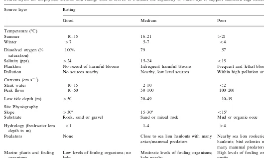
In BCAS, factors within each of these groups are evaluated and categorized into suitability classes (Table 3), following the strategy outlined by Caine (1987). Clearly, the site capability model in BCAS is more comprehensive than the one documented in the first case study (Ross et al., 1993) and provides improved support for assessing finfish aquaculture potential with the caveat that much more data are needed (EAO, 1998). As with shellfish, social and economic factors are not considered in evaluation of sites for finfish aquaculture.
4.3.5. Comments
Among the GIS applications we are aware of in aquaculture, this case study is unique in that: (i) it demonstrates the value of collaborative implementation of such tools and associated spatial databases among multiple governmental organi-zations, a conclusion previously arrived to by Kapetsky and Travaglia (1995); (ii) it is used to both analyze site potential and for routine management (i.e. infor-mation on all aquaculture leases is archived in the databases; see also Arnold et al. (2000), for similar applications of GIS in Florida); and (iii) it is actively used to meet decision support needs of a range of clients.
Increase in the use of BCAS and related information systems in British Co-lumbia has generated debates among policy makers in the province with regard to data ownership/pricing issues (particularly when the tools are being used by private consultants). Such debates are indeed a welcome sign because they demonstrate that use of GIS has progressed beyond the domain of analysts per se, and that these decision support tools are being actively used by decision-mak-ers. A continuing concern among those responsible for collecting and archiving information resources, however, is the degree to which end users are aware of limitations in the databases and analysis tools.
265
Source layers for biophysical criteria, and ratings used in BCAS to evaluate the capability of waterways to support salmonid cage culture
Rating
Plankton Infrequent harmful blooms Frequent and lethal blooms
Pollution No sources nearby Nearby, low level sources Within high pollution areas
Currents (cm s−1)
Substrate Rock, sand or gravel Sand or mixed rock Mud or organic ooze
1–4 \4
B1 Hydrology (freshwater lens
depth in m)
Close to sea lion haulouts with many None
Predators Nearby sea lion rookeries and
haulouts; bird colonies nearby and avian/mammal predators
many mammal predators
High levels of fouling organisms; kelp Low levels of fouling organisms; no
Marine plants and fouling Moderate levels of fouling organisms;
kelp nearby onsite
organisms kelp
Winds and waves/snowfall Site not exposed to polar outflows; Partial exposure to polar outflows; Complete exposure to polar outflows; wave height\1.2 m
wave height 0.6–1.0 m wave heightB0.6 m
and freeze over
4.4.Inland aquaculture potential in Africa (source: Aguilar-Manjarrez and Nath, 1998)
4.4.1.Objecti6es
The motivation for the current study was the pressing need for up-to-date information that can be used to guide aquaculture development in Africa (World Bank, 1996). Recently compiled, more comprehensive spatial databases for the African continent as well as advances in spatial methods to assess fish farming potential provided an additional incentive to conduct the study.
4.4.2. Target decision support audience
The primary audience for continental-scale and country-level estimates of inland aquaculture potential across Africa potentially include national/international tech-nical assistance agencies, large aquaculture corporations, and the international donor community. At this time, however, we are unaware of any instances where the outcomes from the study have actually been used for project assessment or to meet other decision support needs.
4.4.3. Geographic area and scale of analysis
GIS analyses were conducted for the entire African continent, with the exception of Madagascar for which some essential weather datasets were not available. The study examines the extent to which ‘sites’ (essentially areas 5 km×5 km in size corresponding to 3¦ grid cells) satisfy criteria for small-scale and commercial fish farming, and assesses the performance of three index fish species (Nile tilapia, African catfish, and Common carp) under such farming systems.
4.4.4. Analytical methods and results
The basis of the present study is conceptually similar to traditional studies for assessing aquaculture potential (Muir and Kapetsky, 1988; Born et al., 1994). However, use of a GIS greatly enhanced the evaluation, especially with regard to the application of objective decision-making methods, quantifying limitations im-posed by different production factors, providing estimates of the predicted fish farming potential, and visualizing outcomes. GIS analyses were primarily accom-plished using the ArcInfo system, although other software tools (IDRISI, ERDAS and IDA) were also used.
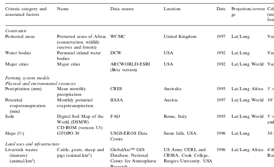
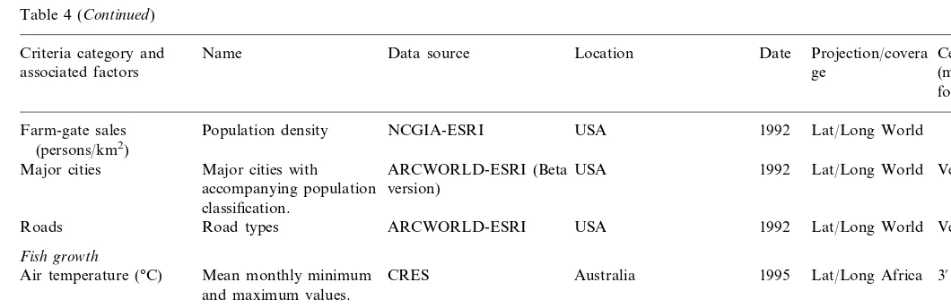
Spatial analysis was limited to assessment of land-based inland aquaculture potential, which for practical purposes implies pond systems. The potential for aquaculture in large inland water bodies (e.g. using cage culture) and in ocean waters was not assessed. This case study provides a good example of data consolidation from multiple sources (Table 4). Analytical procedures in the study were largely derived from previous efforts (Aguilar-Manjarrez, 1996; Kapetsky and Nath, 1997), and involved three phases: