APPLICATION OF 3D SPATIO-TEMPORAL DATA MODELING,
MANAGEMENT, AND ANALYSIS IN DB4GEO
Paul V. Kupera, Martin Breuniga, Mulhim Al-Doorib, Andreas Thomsena
a Geodetic Institute, Karlsruhe Institute of Technology, Karlsruhe, Germany – (paul.kuper, martin.breunig, andreas.thomsen)@kit.edu
bSchool of Engineering, The American University in Dubai, UAE – [email protected]
Commission II, WG II/1
KEY WORDS: Spatio-temporal data modeling, spatio-temporal database, 3D/4D database, geospatial data modeling, geospatial data management.
ABSTRACT:
Many of today´s world wide challenges such as climate change, water supply and transport systems in cities or movements of crowds need spatio-temporal data to be examined in detail. Thus the number of examinations in 3D space dealing with geospatial objects moving in space and time or even changing their shapes in time will rapidly increase in the future. Prominent spatio-temporal applications are subsurface reservoir modeling, water supply after seawater desalination and the development of transport systems in mega cities. All of these applications generate large spatio-temporal data sets. However, the modeling, management and analysis of 3D geo-objects with changing shape and attributes in time still is a challenge for geospatial database architectures. In this article we describe the application of concepts for the modeling, management and analysis of 2.5D and 3D spatial plus 1D temporal objects implemented in DB4GeO, our service-oriented geospatial database architecture. An example application with spatio-temporal data of a landfill, near the city of Osnabrück in Germany demonstrates the usage of the concepts. Finally, an outlook on our future research focusing on new applications with big data analysis in three spatial plus one temporal dimension in the United Arab Emirates, especially the Dubai area, is given.
1. INTRODUCTION AND RELATED WORK
Many of today´s world wide challenges such as climate change (Williams et al., 2010), water supply in mega cities or streams of emigrants are based on spatio-temporal phenomena. Thus geospatial data handling with 3D objects changing in time is a central instrument to support 3D/4D geo-applications with efficient database functionality. Unfortunately, there seems to be no common definition of “3D” in the Geoinformation Science community as many GIS applications are indicated “to be 3D” or “to handle 3D data” though 3D only seems to articulate that the three coordinates x, y and z are used in the geometry of the objects. In this article we distinguish between “3D” space” and “3D objects” as follows:
3D space consists of three dimensions (e.g. x-, y-, z-coordinates for a local coordinate system). In 3D topological space only relative space is relevant and topological relationships are examined between two objects such as disjoint, meet, overlap, covers/coveredBy, inside/contains, equal. No measures e.g. to compute the distance from a point A to a point B exist. However, the “distance” is topologically determined by counting the connected nodes of a graph and determining the sum of the weights for the edges being involved between node A and node B.
Geospatial, i.e. geo-referenced 3D objects are described by their hull (e.g. approximation of the geometry by a closed triangle net) and by their interior (e.g. a tetrahedron net). In opposite to this 2.5 objects only describe surfaces that have no vertical parts and no “overhangs”, i.e. for all points Px,y,z of each object O Pz = f(Px, Py) is true.
Extensive examinations of geo-spatial objects, 3D space, and geo-spatial objects in the field of GIS research have been published e.g. by the group of Peter van Oosterom (van Oosterom and Schenkelaars, 1995), Christine Parent, Stefano Spaccapietra, and Esteban Zimányi (Parent et al. 1999; 2006), (Chen and Zaniolo, 2000), during the Chorochronos project (Koubarakis et al., 2003; Breunig et al., 2003), Helmut Schäben (Schaeben et al., 2003), the groups of Sisi Zlatanova (Khuan et al., 2008; Breunig and Zlatanova, 2011; Xu and Zlatanova, 2013), Jantien Stoter (Stoter et al., 2011), Jacynthe Pouliot (Pouliot et al. 2008;2010; Zamyadi et al., 2014), Thomas Kolbe (Kolbe et al., 2008; Kolbe et al., 2011), Löwner and Becker (Löwner and Becker, 2013), Umit Isikdag (Isikdag, 2014), Alias Abdul Rahman (Duncan and Abdul Rahman, 2015; Azri et al., 2016) and by other authors.
Many approaches have been proposed in literature for spatio-temporal data modeling, especially on changing geometries (e.g. Worboys, 1994; Polthier and Rumpf, 1995; Huisman et al., 2007; van Oosterom and Stoter, 2010). In this article we consider a special case for the representation of 3D object geometries in time which may be likewise used for the modeling of natural and built objects. Furthermore, it cannot only be used for data modeling and data management, but also for data visualization and analysis: are a special case of cell decomposition: we consider the well known simplicial complexes approach, i.e. points / nodes, lines / edges, triangle nets / meshes and tetrahedron nets / meshes are well suited to approximate real world objects and to provide efficient geometric and topological algorithms. Furthermore, topology may be explicitly considered in cell decompositions (Lienhardt, 1991). The decomposition in simplicial complexes is realized with cells of the same type. For
instance, a surface decomposition can be achieved with triangles (2-simplex) and volumetric decomposition with tetrahedrons (3-simplex).
2. 3D PLUS TIME GEOSPATIAL DATA MODELING
In this article we focus on two approaches supporting the modeling of spatio-temporal objects. Whereas the first one concentrates on a clean separation between geometry and topology of the 3D objects, the second enables a continuous change of geometry and a discrete change of the internal topology, i.e. the discretization of the 3D objects.
2.1 Point tube approach
A 4D object describes a continuous phenomenon with a number of discrete time steps. A single time step is formed by a
d-simplicial complex with d ϵ {0,1,2,3}. Adjacent time steps are linked to each other by a linear interpolation.
The Point Tube concept is a special data structure that separates the vertices of a simplicial complex from its net topology. The concept is based on the completeness axioms described by (Egenhofer et al., 1990), i.e. vertices are unique within a simplicial complex. This fundamental idea is also used by the
indexed-face-set procedure which separates the management of vertices from the corresponding mesh of a 3D model. This procedure is i.a. used by various common data formats, such as the OBJ format and the VRML format (Carey and Bell, 1997). Within a single Point Tube, a vertex is clearly identifiable for the entire time series of a 4D object, cf. Figure 1.
Figure 1 - Point Tubes for a model consisting of m vertices.
The movement of these points in space is clearly assigned and can be tracked over time. For the computation of a snapshot that represents the 4D model for a specific date two steps need to be performed:
1. Interpolation of all Point Tubes.
2. Consolidation of the result with the net topology.
Thus, an appropriate 3D model can be created for any point in time, once the date is within the time interval of the 4D model.
2.2 Model by Polthier and Rumpf
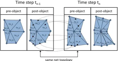
The change of the net topology between two time steps is a critical point for the consistency of a 4D model. However, a change of the net topology at a specific time step is sometimes necessary, for instance to reflect the change of certain regions of the model in detail. The concept of Polthier and Rumpf solves the issue by the introduction of an additional object for the management of 4D models, the so-called pre-object (Polthier and Rumpf, 1994). For every change of the net topology of two adjacent time steps we manage two objects: a pre-object with the net topology top (tn-1) of the previous time step tn-1 and a post-object with the current net topology top (tn) at time step tn. Both objects represent the shape of the geometry of the particular time step tn.
Due to this approach it is possible to have a unique assignment and a 1:1 relationship of individual elements of the model between two time steps. Therefore, it is possible to perform a linear interpolation between these time steps, cf.
Figure 2.
Figure 2 - Two time steps with pre- and post-objects of a 4D model based on 2-simplicial complexes.
The net topology changes at a specific point in time, while the time and therefore the change in geometry is at rest.
2.3 Generalization of the Simplicial Complex Approach for the Modeling of Topology
A well-known discrete approximation of a curved surface is the
triangulation combined with an appropriate interpolation. This can be extended to the discrete representation of 2D-manifolds
in 3D space by triangulated surfaces - a concept that can also be applied to situations such as overhangs, which the simple 2.5D approach cannot handle. It seems thus reasonable to choose an approach to the representation of topology that not only allows for the generalisation of 2.5D triangulated surfaces, but permits the extension towards true 3D models.
To model topology in time we generalize the simplicial complex approach by using larger “units” than only single triangles and tetrahedral: the so-called cellular d-complexes represented by cell-tuple structures (Brisson, 1993) or by the closely related Generalised Maps (G-Maps, Lienhardt 1991) can construct such larger units, i.e. cells. This dimension-independent topological data structure is successfully used since many years in geo-modeling (Mallet, 2002), and especially in the GOCAD 3D modeling and visualization tool (Mallet, 1992). This representation of topology is general, formal and based on a clear and concise mathematical concept, to allow simple algorithms to support topological queries.
In the following we review the significance of G-Maps for geo-modeling (Mallet, 2002; Thomsen et al., 2008). Cellular complexes, and in particular cellular partitions of d-dimensional manifolds (d-CPM) are based on algebraic topology. The topology of d-CPM can be represented by d-dimensional Cell-Tuple Structures (Brisson, 1993) respectively d-dimensional Generalised Maps (d-G-Maps) (Lienhardt, 1991). These possess the combinatorial structure of abstract simplicial complexes, each d-cell-tuple comprising d+1 cells of different dimension, and related to its neighbours by involution operations.
We will now describe how extend oriented G-Maps can be used in 2- and 3-dimensional geospatial databases to support topological operations and queries such as
- systematic traversal by ordered circuits (“orbits”) - boundaries of complex objects
- neighbourhood relationships
- identification of connected components - topological consistency checks
As defined by (Lienhardt, 1991), a d-dimensional Generalized Map (d-G-Map) consists of a finite set of objects called "darts" and a set of one-to-one mappings αi, i= 0,…, d linking pairs of
darts, that are involutions, i.e. that verify αi(αi( x)) = x, and that
further verify the condition
for all i, 0 ≤ i < i+ 2 ≤ j≤d, αiαj is an involution, i. e.
αi(αj(αi(αj(x)))) = x.
Furthermore, the G-Maps are embedded in space by a mapping that to each dart associates a unique combination of a node, an edge, a face, and in 3D a solid in space.
In Brisson’s (1993) terminology, Cell-tuple Structures consist of a set of cell-tuples (node, edge, face, solid) attached to the corresponding spatial objects. The cell-tuples are pairwise linked by "switches" defined by the exchange of exactly one component, which correspond to Lienhardt’s involutions:
α0: (n,e,f,s)Y(n',e,f,s), α1: (n,e,f,s) Y(n,e',f,s),
α2: (n,e,f,s)Y(n,e,f',s), α3: (n,e,f,s)Y (n,e,f,s')
In the following, we use Lienhardt’s terminology with one exception: we do not distinguish between the abstract darts and their practical implementation as cell-tuples, and in consequence systematically use the term cell-tuple instead of
dart.
Cellular complexes can be considered as a generalisation of
simplicial complexes, but lack the algebraic properties of the latter. The involution operations of G-Maps provide cellular complexes with the combinatorial structure of an abstract simplicial complex, where the cells and cell-tuples play the role of abstract nodes and abstract simplexes, while the involution operators define the neighbourhood relationships between the abstract simplexes. It should be noticed that the abstract nodes
n, e, f, s of a G-Map belong to 4 classes distinguished by different dimensions, whereas all nodes of a simplicial complex belong to the same finite set of vertices in space.
3. 3D PLUS TIME GEOSPATIAL DATA MANAGEMENT
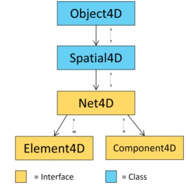
The following implementation of the Point Tube concept as well as the Polthier and Rumpf concept, introduced in Section 2, is based on the object-oriented geo-database architecture DB4GeO (Bär 2007; Breunig et al. 2010;2016). The general structure of the 4D geospatial data management consists of the class Object4D that is composed as described in Figure 3.
Figure 3 - Overview of the structure of an Object4D in DB4GeO.
The actual geometry and topology of a 4D object is contained in a Net4D object that mainly consists of Element4D objects for topological information and Component4D objects for the vertices of a 4D model. For the internal composition of such an object the Point Tube concept and the Polthier and Rumpf concept are used. An explicit workflow is presented in Section 5.2.
3.1 Implementation of the Point Tube Concept
The net topology of a 4D model is managed by a list of
Element4D objects that are realized as Point4D, Segment4D,
Triangle4D or Tetrahedron4D. Such Element4D objects consist of an amount of IDs (1-4, depending on the dimension), that are assigned to individual vertices. The vertices and the implementation of the Point Tube concept are managed in the class Component4D within a list of associative storages
pointTubes (Integer, List < Point3D> ) that are initialized by appropriate importer classes. Thus the net topology and the vertices are clearly separated and each single vertex is traceable within the entire time interval of the 4D model.
3.2 Implementation of Model by Polthier and Rumpf
Within the class Net4D a topologyChange(Date) method was implemented to initialize a net topology change of the 4D model at the specified time. The method
preparePostObject(Date) is used to finalize a preObject and prepare a new postObject. During the finalization process the following steps are performed:
1. The consistency of the current time interval is ensured.
2. A new list of Element4D objects is initialized for the upcoming time interval.
3. New Point Tube data structures are initialized for the upcoming time interval.
Thus it is possible to manage changes of the net topology of a 4D model between adjacent time steps.
3.3 Implementation of G-Maps
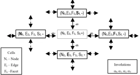
A d-G-Map can be represented as a graph with cell-tuples as nodes and edges defined by the involution operations, cf. Figure
4. Additionally, it can be stored as a relation in tabular form, cf. Figure 5.
Figure 4 - Representation of an oriented 3-G-Map as a graph with symmetries determined by the combinatorial character of
the involutions. Source: (Thomsen et al., 2008)
We require the cellular complexes to be orientable, and the corresponding G-Maps to be oriented. This implies that there are two classes of cell-tuples of the same cardinality, but carrying different polarity. Different from Lienhardt (1991), we exclude the possibility that an involution attaches a cell-tuple to itself (f(x) = x), e.g. at the boundary of the cellular complex. Thus we ensure that involution operations always link pairs of cell-tuples of opposite signs. Instead, we introduce a special non-standard cell, the outside, or “universe”, which in general needs not be simply connected and may comprise holes and islands, and provide the universe also with cell-tuples and involutions on the boundary.
Figure 5 - Representation of an oriented 3-G-Map as a relation with additional symmetry constraints determined by the combinatorial character of the involutions. Source: (Thomsen et
al., 2008)
Though this approach augments the numbers of objects to be handled, it simplifies needed operations and algorithms on the G-Maps.
3.3.1 Operations on G-Maps: Navigation on the G-Map
Orbits. By definition, the repeated application of the same involution i, means cycling between the two states i(x) and
x=i(i(x)). If we combine two or more different involutions i, j, …, the picture changes: i(j(x)) in general cannot
expected to coincide neither with x nor with j(i(x)). However,
Lienhardt’s definition of a d-G-Map (see above) implies that (x)= 0(2(x)) is an involution for dimension d = 2 and d = 3,
as are
(x)= 0(3(x)) and δ(x)= 1(3(x)) for d = 3.
An orbit in a G-Map is defined as the maximal subset of d-cell-tuples that can be reached from a start d-cell-tuple cts by any combination of a given subset of the involutions 0 …d. Let us note such an orbit orbitd( cts,
i,...j) or shorter
orbitdi…j(cts).
Singletons {cts} and pairs { cts,ai(cts)} may be considered as the
result of trivial orbits. In 2D, non-trivial orbits are:
- orbit2
01(cts) enumerates the cell-tuples associated with a face
- orbit2
02(cts) enumerates the cell-tuples associated with an edge
- orbit2
12(cts) enumerates the cell-tuples associated with a node
- orbit2
012(cts) enumerates all cell-tuples of the connected
component containing cts.
In 3D, the following classes of non-trivial orbits exist:
- orbit3
01(cts), orbit302(cts), orbit303(cts), orbit312(cts),
orbit3
13(cts), orbit323(cts)
- orbit3
012(cts), orbit3013(cts), orbit3023(cts), orbit3123(cts)
enumerate the cell-tuples associated with a solid, face, edge,
node n, respectively.
- orbit3
123(cts) enumerates all cell-tuples of the connected
component containing cts.
By marking each cell that has once been encountered, and successively skipping marked cells, we can use orbits to enumerate all cells of a given type encountered on the way. Most of these orbits can be implemented using nested simple programming loops, except for the following ones: orbit2
012(),
orbit3
012(), orbit3123(), orbit30123(). These can be implemented
recursively e.g. as depth-first search using a stack (Lévy, 1999). This approach has a shortcoming: whereas non-recursive implementations yield sequences of cell-tuples that form a continuous path in the Graph structure representation of the G-Map, recursively implemented orbits yield sequences that may comprise discontinuities when the procedure is forced to backtrack. We are therefore currently investigating to what extent these orbits can be implemented as continuous closed loops.
Loops. For the basic split operation on 3-cells (solids) described below, we need to define a closed loop of cell-tuples on the inner surface of the solid, i.e. a sequence of the form
ct0–i0 –… - ik-1 - ctk–ik -…iN-1– ct0,
passing from each cell-tuple ctk to the next by an involution ik.
This sequence may be user-defined rather than generated by an orbit. Once it has been defined, e.g. as a linked list, it is easy to use an iterator to produce the sequence of cell-tuples in similar fashion as by an orbit. On the other hand, an orbit that does not
make any “jumps” produces a continuous loop of cell-tuples that can be stored in form of a loop. It can be represented in condensed form, either as a start cell-tuple followed by a sequence of pairwise adjacent cell-tuples, or followed by a sequence of involution selectors i = 0, 1, 2 ,3, that at each step determine the next involution to follow. Obviously it takes at most 4 bits to encode such a selector. A possible external representation is a start cell-tuple ct0(n0,e0,f0 s0) followed by a
sequence of cells ci, where each transition ki from cell-tuple
cti(ni,ei,fi,si) to the next is defined by exchanging ci against the
corresponding cell in cti.
Orbits and loop iterators are used to traverse connected subsets of a d-G-Map. They are instantiated with a start cell-tuple, and in the case of loop iterators with the sequence of involution selectors. Methods are .hasNext(), .getNext(), .hasPrevious(), .getPrevious(), .size(), and .restart().
The introduced operations on G-Maps for topological navigation can be extended in time straight forward by considering the topology at single time steps or at a certain time interval. In the latter case interpolation and the Model by Polthier and Rumpf (1995) may be applied.
4. 3D PLUS TIME GEOSPATIAL ANALYSIS
In this article only simple geometric and topological data analysis operations based on time-dependent data are discussed. They are tailored to the operations already implemented in DB4GeO and the application presented in chapter 5. I.e. geometric objects are supposed to be implemented as approximated linear objects in the shape of simplicial complexes. They are based on simplexes being topologically classified in the usual way, i.e. towards their dimension: 0-simplex = node, 1-simplex = edge, 2-simplex=triangle, 3-simplex=tetrahedron. We introduce the following typical geometric and topological operations on spatio-temporal data:
calculateHull(A, T)
Calculates the hull of a 3D object A during a time interval T, i.e. the boundary of the solid which consists of a closed 2-simplicial complex, i.e. a closed triangle net. It returns the constant hull, i.e. discretization of the triangle net bounding the solid A in the time interval T(tstart, tend).
averageSpeed(A, T)
Calculates the average speed of a 3D object A during a time interval T. It returns a real value indicating the average speed of 3D object A during the time interval T(tstart, tend).
4D-to-3D service(A, tx)
Calculates a certain snapshot of a 4D object (3D plus time). It returns the geometry of 4D object A at time step tx.
minDistance(A, B, T)
This operation computes and returns the minimum distance between the bounding box of two 3D objects A and B within the time interval T.
maxDistance(A, B, T)
This operation computes and returns the maximum distance between the bounding box of two 3D objects A and B within the time interval T.
intersection(VP, {A}, T)
Calculates the intersecting geometry between a vertical plane
VP and a set {A} of 3D objects within the time interval T. It returns a list of pairs, each consisting of a constant intersecting geometry between the vertical plane VP and the set {S} of 3D objects and a time interval (tstart, tend).
testTopo(A, S, T)
Determines the topological relationship (disjoint, meet, covers/coveredBy, overlap, inside/contains, equal) between a 3D object A and a 3-simplex S between a time interval T. It returns a list of pairs, each consisting of a Boolean value and a time interval (tstart, tend).
As we see in the above list of spatio-temporal operations they refer either to a single 3D object (calculateHull, averageSpeed, 4D-to-3D service) or they serve as binary operations between two 3D objects (distance) or they need a single 3D object plus an auxiliary object (such as vertical plane, set of 3D objects, simplex) as input data (intersection, testTopo).
5. APPLICATION EXAMPLE IN DB4GEO
5.1 Review of DB4GeO
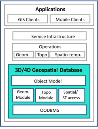
The service-based geospatial database architecture DB4GeO (Bär 2007, Breunig et al. 2010; 2016) is fully implemented in the Java programming language providing data access via the REST specification (Fielding, 2000), a Web Feature Service (WFS), and a prototypical Web Processing Service (WPS) as standardized by the Open Geospatial Consortium (OGC). DB4GeO has already been tested to demonstrate several topological (Thomsen et al. 2008), geospatial and spatio-temporal geo-applications (Breunig et al., 2016). Figure 6 reviews the current system architecture of DB4GeO. Based on an object-oriented database management system (OODBMS) modules for geometric and topological modeling, as well as for spatial and spatio-temporal data access, are implemented. Upon the object model the operations for geometric, topological, and spatio-temporal are realized. They are partwise accessible via the service infrastructure, e.g. DB4GeO offers several geometric and topological web services as introduced in Chapter 4.
Figure 6 - System architecture of DB4GeO.
Finally, GIS clients may access the 3D/4D geospatial database via its web services or directly via the REST interface.
5.2 Piesberg Application
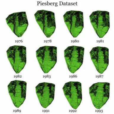
5.2.1 Description of the application and the data: The usage of the described concepts is demonstrated based on an exemplary data set. Therefore, appropriate spatio-temporal data is required. A suitable scenario is the modelling of the continuous change of a region over a certain period of time. The data set of the Piesberg landfill site in Osnabrück offers such a data base (Lautenbach and Berlekamp, 2002; Butwilowski, 2015). From 1976 to 1993 in total 12 models of the Piesberg were developed. They describe the continuous transformation of the region, cf. Figure 7.
Figure 7 - Piesberg dataset with 12 time steps from 1976 to 1993. Source: (Butwilowski, 2015)
Each 3D model of the Piesberg dataset corresponds to a discrete time step within the time interval from 1976 to 1993 and consists of 19k to 30k triangles.
5.2.2 Data Modeling: In DB4GeO the discrete time steps of the Piesberg dataset can be combined to a comprehensive 4D model that represents the continuous change of the Piesberg. For the construction of such a 4D model in DB4GeO the Point Tube concept is used by appropriate import classes, i.e.
GocadImporter4D. Thereby the triangles are separated from the vertices of the dataset. The net topology of the Piesberg changes with every time step. Therefore, the concept of Polthier and Rumpf is used to manage the dataset by the use of pre- and
post-objects. Thus the Point Tube data structures are valid between a post- and pre-object. Intermediate states of the model are computed by a linear interpolation.
5.2.3 Data Management: The composition of the 4D model of the Piesberg is divided into multiple steps. First, the import class GocadImporter4D is applied on the 3D model of the initial time step of the dataset, i.e. 1976. Thereby the 4D model is initialized with an appropriate amount of Point Tube data structures and an initial net topology. In the following, the subsequent steps of the dataset are added to extend the 4D model, cf. Figure 8.
Figure 8 - 4D model of the Piesberg.
Since the net topology changes with every time step, the
topologyChange(Date) method is called to finalize the
preObject and prepare a new postObject. This procedure is repeated with every time step of the dataset. Afterwards the comprehensive 4D model is ready to be used for data-retrieval operations and spatial or spatio-temporal analysis. In the further progress, the 4D model of the Piesberg as well as other 4D models can be easily extended with additional time steps.
5.2.4 Data Analysis: Due to the previous steps, the Piesberg dataset is managed in a single consolidated Object4D. Thus data analysis operations such as averageSpeed and the 4D-to-3D service are performed directly at the 4D model. For instance, the operation 4D-to-3D service (piesberg, 1989-01-01T00:00:00) results in a 3D object that represents the Piesberg for the time 1989-01-01T00:00:00. Further operations presented in Section 4 along with an appropriate visualization of the results are planned to be implemented in the near future.
6. CONCLUSIONS AND OUTLOOK
In this article we have described the application of concepts for the modeling, management, and analysis of geospatial data with 2.5 and 3 spatial dimensions, respectively, plus one temporal dimension implemented in DB4GeO, our service-oriented geospatial database architecture. The modeling of spatio-temporal data allows the change of geometry and internal topology (discretization) of the objects in continuous time. Thus database queries not only on previously stored states of geospatial data models are provided but also “in between queries”, i.e. on interpolated time intervals in between two time steps. Finally, simple geometric and topological analysis operations are presented.
In our DB4GeO research group we will further optimize the system e.g. regarding the management of arbitrary parameters including space and time. Furthermore, we intend to focus on big data challenges of the Middle East such as World Expo 2020 in Dubai, Dubai Smart City or soccer world cup 2022 in neighboring Qatar. There is a huge amount of possible applications for spatio-temporal data handling: As advancement of technology drives forward the Internet of Everything, organizations will see expanding information from wearable and cell phones, services profiling in big sports events as stadiums will be able to use information gathered at sport events using a large number of sensors in Dubai Smart City. Showing the requirement for Big Data arrangements in the area, 40
percent of business pioneers referred to information elucidation as the greatest hindrance to conveying significant bits of knowledge. The Middle East and Africa will post the world's speediest versatile information activity development, according to Cisco's Visual Networking Index, 2013-2018. Therefore the area is very much set to influence and contribute to improved connectivity and handling of Big Data.
In the field of water supply in Dubai, a local project has demonstrated proof of how landscapes help in modifying the microclimate of Dubai specifically temperature decrease by making rich scenes for diminished temperatures. The undertaking used a 3D/4D numerical model utilizing a 3-dimensional non-hydrostatic microclimate model that can figure and reproduce atmosphere in urban regions with sever weather. The capacity and opportunity, in any case, for a multi-disciplinary project group, including administration, to effortlessly search, audit and envision last cross-discipline study results in a quick, responsive and effectively comprehendible way is a challenge for further research. In the transport world, and as a part of the UAE Intelligent Transport framework (ITS), arrangement 2030 is a new strategy to support the transport infrastructure developments taking place, to help the Emirates accomplish its objective to construct a world-class transport framework. In the tendering phase portable message signs, incident-detection stations, non-citation traffic cameras and a web-based traffic congestion information service are examined that all are suitable use cases for the analysis of big spatio-2016. Classified and clustered data constellation: An efficient approach of 3D urban data management. In: ISPRS Journal of Photogrammetry and Remote Sensing, pp. 30-42.
Bär, W., 2007. Managment of geo-scientific 3D data in mobile database systems (in German). Ph.D. Thesis, University of Osnabrück, Germany.
Brission, E., 1993. Representing Geometric Structures in d Dimensions: Topology and Order. In: Discrete & Computational Geometry 9, pp. 387-426.
Breunig, M., Kuper, P.V., Butwilowski, E., Thomsen, A., Jahn, M., Dittrich, A., Al-Doori, M., Golovko, D., Menninghaus, M, 2016. The Story of DB4GeO - A Service-Based Geodatabase Architecture to Support Multi-Dimensional Data Analysis and Visualization.In: ISPRS Journal, in print, 19 p.
Breunig, M., Schilberg, B., Thomsen, A., Kuper, P.V., Jahn, M., Butwilowski, E., 2010. DB4GeO, a 3D/4D geodatabase and its application for the analysis of landslides. Geographic Information and Cartography for Risk and Crisis Management.
Lecture Notes in Geoinformation and Cartography, Springer, Heidelberg, pp. 83-102.
Breunig, M., Türker, C., Böhlen, H., Dieker, S., Güting R.H., Jensen, C.S., Relly, L., Rigaux, P., Schek, H.J., Scholl, M., 2003. Architecture and Implementations of Spatio-Temporal Database Management Systems.In: Spatio-Temporal Databases – The CHOROCHRONOS Approach. Lecture Notes in Computer Science Vol. 2520, Springer-Verlag, Heidelberg, pp. 219-264. Breunig, M., Zlatanova, S., 2011. 3D geo-database research: Retrospective and future directions, In: Computers & Geosciences, Volume 37, 7, pp. 791-803.
Butwilowski E., 2015. 3D data and model management for the geosciences with particular emphasis on topology and time, PhD thesis, Karlsruhe Institute of Technology.
Carey R., Bell G., 1997. The Annotated VRML 2.0 Reference Manual, Essex, UK, Addison-Wesley Longman Ltd., 1997. Chen, C.X., Zaniolo, C.: SQLST, 2000. A Spatio-temporal Data Model and Query Language. Proceedings of the 19th International Conference on Conceptual Modeling, Salt Lake City, Utah, USA, pp. 96-111.
Duncan, E.E., Abdul Rahman, A., 2015. 3D GIS for mine development – integrated concepts. In: International Journal of Mining, Reclamation and Environment, 29, 1, pp. 3-18.
Egenhofer M. J., Frank A. U., Jackson J. P., 1990. A Topological Data Model for Spatial Databases, Proceedings of the First Symposium on Design and Implementation of Large Spatial Databases, New York, NY, USA, pp. 271–286. Fielding, R.Th., 2000. Achitectural styles and the design of network-based software architectures, Ph.D. thesis, University of California, Irvine, USA (2000) 15.
Huisman, O., Forer, P., McDowall, C., 2007. The Nature of Prisms: Exploring Data Quality and Vagueness in Dynamic Spatio-Temporal Constructs, In: Proceedings of the 5th International symposium on Spatial Data Quality SDQ 2007, Modelling qualities in space and time, ITC, Enschede, The Netherlands, 13-15 June, 2007. Enschede : ITC, 2007. 7 p.
Isikdag, U., 2014. Innovations in 3D Geoinformation Sciences (ed.), Lecture Notes in Geoinformation and Cartography, Springer, Heidelberg, 319p.
Khuan, C.T., Abdul Rahman, A., Zlatanova, S., 2008. 3D solids and their management in DBMS, In: Van Oosterom, Zlatanova, Penninga&Fendel (Eds,), Advances in 3D Geoinformation Systems, Lecture Notes in Geoinformation and Cartography, Springer-Verlag, Heidelberg, pp. 279-313.
Koubarakis, M., Sellis, T., Frank, A.U., Grumbach, S., Güting, R.H., Jensen, C.S., Lorentzos, N., Manolopoulos, Y., Nardelli, E., Pernici, B., Schek, H.-J., Scholl, M., Theodoulidis, B., Tryfona, N. (Eds.), 2003. Spatio-Temporal Databases – The Chorochronos Approach, Lecture Notes in Computer Science,
Vol. 2520, Springer-Verlag, Heidelberg,
Kolbe, T. H., 2008. Representing and Exchanging 3D City Models with CityGML. In: Lee, Jiyeong / Zlatanova, Sisi (Hg.):
Proceedings of the 3rd International Workshop on 3D Geo-Information, Seoul, Korea. Lecture Notes in Geoinformation & Cartography, Springer Verlag.
Kolbe, Th. H., König, G., Nagel, C. (eds.): Advances in 3D Geo-Information Sciences. Lecture Notes in Geoinformation and Cartography. Springer, 2011.
Lienhardt, P., 1991. Topological Models for Boundary Representation: a Comparison with n-dimensional Generalized Maps. Computer Aided Design 23(1), pp. 59-82.
Löwner, M.-O., Becker, T., 2013: A topological framework for the temporal aspects of landform development. ISPRS Ann. Photogramm. Remote Sens. Spatial Inf. Sci., II-2/W1, 237-246, doi:10.5194/isprsannals-II-2-W1-237-2013, 10p.
Mallet, J.L., 1992. GOCAD: a Computer Aided Design Programme for Geological Applications. Turner A.K. (Ed.), Three-Dimensional Modelling with Geoscientific Information Systems. Proceedings of NATO ASI 354, Kluwer Academic Publishers, Dordrecht, pp. 123-142.
Mallet, J.L., 2002. Geomodelling. Oxford University Press, 599 p.
Parent, C., Spaccapietra, S., Zimányi, E., 1999. Spatio-Temporal Conceptual Models: Data Structures + Space + Time. In: Proceedings GIS´99, Proceedings of the 7th ACM International Symposium on Advances in Geographic Information Systems, New York, pp. 26-33.
Parent, C., Spaccapietra, S., Zimányi, E., 2006. Conceptual Modeling for Traditional and Spatio-Temporal Applications – The MADS Approach, Springer.
Polthier, K., Rumpf, M., 1995. A Concept for Time-Dependent Processes. In: Visualization in Scientific Computing, Springer, Heidelberg, pp. 137-153.
Pouliot, J., Badard, T., Desgagné, E., Thomas, V. 2008. Development of a Web Geological Feature Server (WGFS) for sharing and querying of 3D objects. 2nd International Workshop on 3D Geo-Information, December 14-16, Delft, Netherlands, 115-130.
Pouliot, J., Roy, T., Fouquet-Asselin, G., Desgroseilliers, J., 2010. 3D Cadastre in the province of Quebec: A first experiment for the construction of a volumetric representation.
In: Advances in 3DGeo-Information Sciences. Lecture Notes in Geoinformation and Cartography, Volume Editor(s): Kolbe, Thomas H.; König, Gerhard; Nagel, Claus. 3DGeoInfo conference, Berlin, Nov. 3-4., pp. 149-162.
Schaeben, H., Apel, M., v.d. Boogart, G., Kroner, U., 2003. GIS 2D, 3D, 4D, nD. Informatik Spektrum, Vol. 26, No. 3, June 2003, pp. 173-179.
Stoter, J., G. Vosselman, J.Goos, S. Zlatanova, E. Verbree, R. Kloosterand M. Reuvers, 2011. Towards a National 3D Spatial Data Infrastructure: Case of The Netherlands, In:
Geoinformation: Organ der Deutschen Gesellschaft für Photogrammetrie und Fernerkundung e V. 2011, 6, pp. 405-420.
Lautenbach S., Berlekamp J., 2002. Datensatz zur Visualisierung der Zentraldeponie Piesberg in Osnabrück, University of Osnabrück.
Polthier K., Rumpf M., 1994. A concept for Time-Dependent Processes, Goebel et al., (Eds), Visualization in Scientific Computing, Springer, Vienna, pp. 137-153.
Thomsen, A., Breunig, M., Butwilowski, E., Broscheit, B., 2008. Modelling and managing topology in 3D geoinformation systems. Proceedings of 3D Geoinfo 07, Delft, Advances in 3D Geoinformation Systems, Lecture Notes in Geoinformation and Cartograhphy, Springer, Heidelberg, pp. 229-246.
van Oosterom, P., Schenkelaars, V., 1995. The development of an interactive multi-scale GIS. International Journal of Geographical Information Systems 9(5), (1995), pp. 489-507.
van Oosterom, P., Stoter, J.E., 2010. 5D Data Modelling: Full Integration of 2D/3D Space, Time and Scale Dimensions.
GIScience 2010, pp. 310-324.
Worboys, M., 1994. A Unified Model for Spatial and Temporal Information. The Computer Journal, 37(1), pp. 25–34.
Williams, M., Cornford, D., Bastin, L., Jones, R. and Parker, S.:, 2010. Automatic processing, quality assurance and serving of real-time weather data. Computers and Geosciences, 37, 3, (2010), pp. 353-362.
Xu, D., Zlatanova, S., 2013. Am approach to develop 3D GeoDBMS topological operators by reducing existing 2D operators, ISPRS Annals – Volume II-2/W1, 2013, WG II/2, 8th 3D GeoInfo Conference & ISPRS WG II/2 Workshop, 291–298 November 2013, Istanbul, Turkey.
Zamyadi A, Pouliot J, Bédard Y, 2014. Towards 3D Metadata for Discovering 3D Geospatial Models, In: Innovations in 3D Geo-Information Sciences, Springer Berlin Heidelberg, Lecture Notes in Geoinformation and Cartography, pp. 267-290.