3D BUILDING RECONSTRUCTION FROM LIDAR POINT CLOUDS BY ADAPTIVE
DUAL CONTOURING
E. Orthubera, b, J. Avbelja∗ a
German Aerospace Center, Oberpfaffenhofen, D-82234 Wessling - [email protected]
bDept. of Remote Sensing Technology, Technische Universitaet Muenchen, Arcisstr. 21, D-80333 Muenchen
KEY WORDS:LIDAR, Building, City, Model, Reconstruction, Computer, Vision, Photogrammetry
ABSTRACT:
This paper presents a novel workflow for data-driven building reconstruction from Light Detection and Ranging (LiDAR) point clouds. The method comprises building extraction, a detailed roof segmentation using region growing with adaptive thresholds, segment bound-ary creation, and a structural 3D building reconstruction approach using adaptive 2.5D Dual Contouring. First, a 2D-grid is overlain on the segmented point cloud. Second, in each grid cell 3D vertices of the building model are estimated from the corresponding LiDAR points. Then, the number of 3D vertices is reduced in a quad-tree collapsing procedure, and the remaining vertices are connected according to their adjacency in the grid. Roof segments are represented by a Triangular Irregular Network (TIN) and are connected to each other by common vertices or - at height discrepancies - by vertical walls. Resulting 3D building models show a very high accuracy and level of detail, including roof superstructures such as dormers. The workflow is tested and evaluated for two data sets, using the evaluation method and test data of the “ISPRS Test Project on Urban Classification and 3D Building Reconstruction” (Rottensteiner et al., 2012). Results show that the proposed method is comparable with the state of the art approaches, and outperforms them regarding undersegmentation and completeness of the scene reconstruction.
1. INTRODUCTION
1.1 Motivation
For more than two decades, 3D building reconstruction has been an active research topic of remote sensing, photogrammetry, and computer vision (Rottensteiner et al., 2012; Wang, 2013; Haala and Kada, 2010; Lafarge and Mallet, 2012). Continuing research is driven by the increasing demand for accurate, automatically produced, and detailed 3D city models (Wang, 2013). City mod-els are used for urban planning (Verma et al., 2006), change de-tection (Rau and Lin, 2011) and environmental or telecommuni-cation simulations (Geibel and Stilla, 2000; Rau and Lin, 2011). Today’s utilization of city models expands to everyday user-driven mobile applications, such as location based services (Wang, 2013; Brenner, 2005), 3D Geographic Information Systems (GIS) for navigation, driver assistance systems, virtual tourism (Zhou and Neumann, 2010), and augmented reality. The effort for keeping 3D city models up-to-date depends on the level of automation in building reconstruction.
LiDAR point clouds are well suited for automatic building recon-struction. In comparison to optical stereo imagery, where stereo matching is needed to obtain 3D geometry, LiDAR data con-tains directly measured, and thus very accurate 3D information (Meng et al., 2010; Haala and Kada, 2010). With continuously increasing LiDAR sensor capacities and point densities, research on building reconstruction has set a focus on LiDAR point clouds (Geibel and Stilla, 2000; Haala and Kada, 2010).
1.2 Related Work
Building reconstruction requires the extraction of individual build-ings’ points from a LiDAR scene. Once buidlings are extracted, there are two main approaches to reconstruction, i.e. model- and data-driven approaches.
∗Corresponding author
Model-drivenapproaches select for each building point cloud, or
parts of it the best fitting parametric model and its corresponding parameters from a predefined catalogue (Maas and Vosselman, 1999; Vosselman and Dijkman, 2001; Kada and McKinley, 2009; Haala and Kada, 2010; Zhang et al., 2012). Model-driven restruction is robust, effective and fast, because regularization con-straints, such as parallelity and orthogonality, are already inherent in the parametric models. However model-driven approaches are limited to the beforehand defined model portfolio and are there-fore not flexible to model all roof shapes.
Data-drivenapproaches connect individual roof segments, which
are constructed according to a preliminary segmentation of the building point cloud. Even though data-driven approaches re-quire a high effort for subsequent regularization, they are widely used (e.g. Rottensteiner et al., 2012; Wang, 2013). The advan-tages of these approaches are a high fit to the input data and flexibility in modeling complex roof shapes. Roof segmentation can be achieved by surface-fitting techniques such as RANSAC (Sohn et al., 2008; Tarsha-Kurdi et al., 2008; Brenner, 2000) or Hough transform (Vosselman and Dijkman, 2001; Sohn et al., 2012; Vosselman et al., 2004), or using region growing meth-ods (Rottensteiner, 2003; Oude Elberink and Vosselman, 2009; Perera et al., 2012; Verma et al., 2006; Nurunnabi et al., 2012; Dorninger and Pfeifer, 2008; Lafarge and Mallet, 2012). Typi-cally, each segment is delimited by a polygonal segment bound-ary, which is created by using e.g. Alpha-shapes (Dorninger and Pfeifer, 2008; Kada and Wichmann, 2012; Sampath and Shan, 2007; Wang and Shan, 2009), the Voronoi neighborhood (Maas and Vosselman, 1999; Matei et al., 2008; Rottensteiner, 2003) or using a 2D-grid-cell projection (Sun and Salvaggio, 2013; Zhou and Neumann, 2008). Polyhedral 3D models are commonly con-structed on the basis of heuristics for extracting and connecting 3D lines along the segment boundaries (Dorninger and Pfeifer, 2008; Vosselman and Dijkman, 2001; Sohn et al., 2008; Rau and Lin, 2011; Rottensteiner, 2003). Structural modeling procedures estimate the coordinates of the building model’s 3D vertices by error propagation techniques (Lafarge and Mallet, 2012) or
cal error minimization (Fiocco et al., 2005) are less frequently used. The latter technique is also used by Zhou and Neumann (2010), who apply a 2.5D dual contouring algorithm on a point cloud which is segmented into different height layers. The asset of their method is the outstanding flexibility to model complex roof shapes, including non-planar roof segments. However, the algorithm cannot create step edges between roof segments con-necting within one roof height layer, which results in a deficiency for modeling superstructures.
2. METHOD
The proposed workflow (Fig. 1) adapts the method of Zhou and Neumann (2010) for modeling superstructures. The algorithm is modified for a situation-adaptive estimation of the 3D building model’s vertices from a detailed roof segmentation.
Input to the procedure are LiDAR data, clustered into sets of Li-DAR points representing different buildings, hereafter referred to as building point clouds. First, the roof points are segmented on the basis of Triangulated Irregular Network (TIN) of the data. Second, a boundary polygon is created for each segmented clus-ter. Third, vertices of the 3D building model are estimated and connected using an adaptive 2.5D Dual Contouring procedure. Regularization for enhancing model simplicity is not included in this is work.
...Roof.segmentation:. Robust.TIN3Region.Growing
Segment.boundaries.creation
Modeling:.Adaptive.2'5D.Dual.Contouring
Quadtree.collapsing. Grid.data.creation
Adaptive.QEF>.construction.F.minimization
QEF>.residual. ...>.thr?
3D.building.model*s.vertices no
yes
Connect.vertices.to.roof.triangles.F.walls
Watertight.3D.building.model LiDAR.building.point.cloud
Figure 1. Overview of the proposed workflow for 3D building model reconstruction from LiDAR point clouds. QEF abbrevia-tion stands for Quadratic Error Funcabbrevia-tion (Eq. (4)).
2.1 Roof Segmentation
The goal of roof segmentation is to cluster the points according to the roof segments they belong to. While most region grow-ing (RG) segmentation techniques assume roof segments to be planar, the proposed segmentation is designed to allow any con-tinuous shape. For this purpose, a robust TIN-based RG tech-nique is proposed. Moreover, in contrast to most RG techtech-niques (e.g. Dorninger and Pfeifer, 2008; Oude Elberink and Vossel-man, 2009; Sampath and Shan, 2010; Sun and Salvaggio, 2013), the proposed method does not assign one segment label to each LiDAR point, but to each triangle of the TIN. Thereby, LiDAR points, which are part of differently labelled triangles, have more than one label. The labelling of triangles minimizes gaps between
adjacent intersecting roof segments and allows accurate boundary determination.
The RG procedure iteratively starts at seed triangles defined by a minimum Local Unevenness Factor (LU F), defined as
LU Ft=
Kt
X
k
Ak
Kt
P
k
Ak
·mean
nx,k−n¯x ny,k−n¯y nz,k−n¯z
, (1)
whereAkis equal to the area andnk = [nx,k, ny,k, nz,k]Tis
the normal of thek-th ofKt triangles which are in the
neigh-borhood of trianglet;n¯x/y/zare the means of allnx/y/z,k. For
RG, each triangle is tested for a fixed threshold on the local angu-lar deviation and for two adaptive thresholds. These two robust adaptive thresholds are built according to Nurunnabi et al. (2012) and are using theLU F and the LiDAR points’ distances to the current best fitting segment plane.
2.2 Segment Boundaries
For each point cloud representing a roof segment, a polygonal boundary is created in an iterative convex-hull collapsing proce-dure. Iteratively, each line segments of the convex hull is refined by the LiDAR point with a minimum distance measure. The refinement stops when the line segment is shorter than a direc-tionally dependent threshold, which is created by considering the LiDAR point spacings in across-track and along-track sampling directions.
2.3 Building Modeling
The proposed modeling algorithm estimates and connects the 3D vertices of the building model using an adaptive 2.5D Dual Con-touring procedure. In section 2.3.1, the 2.5D dual conCon-touring principle is introduced. A 2D grid is overlain on the data, and grid data is computed (section 2.3.2). In an iterative quadtree collapsing procedure, a Quadratic Error Function (QEF) is con-structed from the grid data of each four adjacent grid cells. The minimization of the situation-adaptive QEF results in the coordi-nates of one or more 3D vertices of the building model, depend-ing on whether the vertices represent a step- or an intersection edge (section 2.3.3).
2.3.1 Dual Contouring principle For building reconstruction, a 2D grid is overlain to the segmented LiDAR points in the x-y-plane. The Dual Contouring principle can be illustrated by the example of estimating the vertices of boundary polygons, which separate the segments in the 2D-plane. In each grid cell, a poly-gon vertex is estimated by minimizing its distances from local boundary lines, which separate the LiDAR points of different seg-ments. Then, a polygon is created by connecting the vertices of adjacent cells (Fig. 2).
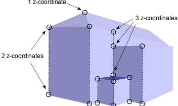
The purpose of 2.5D Dual Contouring is to estimate vertices of the 3D building polygon in each grid cell, which are described by so-called hyperpoints. Depending on whether a hyperpoint
X =
x y zv zv+1 ... zVTdescribes a step edge or
an intersection edge, it contains two or more 3D vertices with the same x-y-coordinates, but with different coordinates. Each z-coordinate defines a 3D vertexX3D,v = [x, y, zv], in which all
segmentsSkwithin a local height layerHvintersect (Fig. 3).
A hyperpoint’s optimal xandy-coordinates minimize the 2D-distancesE2D(X)to local boundary lines (LBL) between the
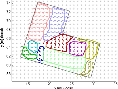
(a) 2D-grid overlain to segmented point cloud. Each colour repre-sents one segment.
(b) Blue lines represent local boundary lines for each pair of segments in a cell.
(c) QEF minimization (blue cell) using all local boundary lines from adjacent cells (pink lines). The yellow star is the QEF solution, i.e. one optimal vertex of the polygo-nal boundary line.
(d) QEF solutions (yellow stars) are computed for all cells and con-nected to the polygonal boundary line (black line) according to their adjacency in the grid.
Figure 2. 2D Illustration of the Dual Contouring principle. The input is segmented point cloud (a) and the QEF solutions are the polygonal boundary lines (d).
1 z-coordinate
2 z-coordinates
3 z-coordinates
Figure 3. Hyperpoints at intersection edges (one z-coordinate) and step edges (more than one z-coordinate).
E2D(X) =
Additionally, an optimal 3D vertexX3D,vcorresponding toHv,
v = (1, ..., V)minimizes the 3D-distancesE3D(X)to the
lo-cal surface planes (LSP), which are fitted to the LiDAR points belonging to each segmentSk,k= (1, ..., M).E3D(X)is
com-wheremjk is thej-th normal of the local surface planeLSPk
on segmentSk, andqjkis a point on this plane.
CombiningE2D(X)(Eq. 3) andE3D(X)(Eq. 2), each
hyper-point is estimated by minimizing the Quadratic Error Function (QEF) (Zhou and Neumann, 2010)
ˆ
X= argmin
X {E2D(X) +E3D(X)}. (4)
2.3.2 Local grid data For each vertex of the 2D grid, a lo-cal surface planeLSP = [m, q]is determined, wherem = [mx, my, mz]Tis the plane’s normal, andq= [qx, qy, qz]Tis
a point on the plane.qxy= [qx, qy]Tis equal to the grid vertex.
EachLSPis associated with a segment labellLSP, according to
the segment, which is the closest toqxy(Fig. 4 b). Vectorm
is determined by averaging the normals of theKnearest TIN-triangles belonging toSk.
For each grid cell, a local boundary lineLBLk,l= [n,p]is
esti-mated for each pair of segmentsSkandSlusing a Least Squares
approach (Fig. 4 a).LBLk,lis estimated from all LiDAR points
belonging toSkandSl, which are within a buffer zone around
the grid cell. LBLwhich have no intersection pointpwith the grid cell’s border are discarded.
2.3.3 Adaptive QEF In contrast to
Zhou and Neumann (2010), whose building point cloud is seg-mented into different height layers, the presented method works on a detailed segmentation of the roof into diffent segments. While Zhou and Neumann (2010) estimate one z-coordinate for each global roof height layer, (eq. 4), the proposed method requires that the LiDAR points within one cell are grouped into local height layers. The advantage of local height layers is that step edges can be created between segments from one global roof height layer. This allows to model complex roof structures such as dormers and shed roof segments. Grouping the segments into local height layersHvis achieved by estimating a step edge
prob-abilitySEPfor each local boundary lineLBL(Eq. 5). Within one cell, all segments with an SEP < 0.5are grouped into one local height layerHv. Assuming the z-coordinates of
Li-DAR points to be normally distributed around their true value, the equation for computing SEP is designed to use the minimum step edge heightTstepas standard deviation:
SEP = exp
whereTstepis a fixed step edge threshold anddza measure
ex-pressing the local height difference of the two segments.
In Zhou and Neumann (2010), all local boundary linesLBL rep-resent step edges, as their input point cloud is only segmented into global roof height layers. When constructing the QEF, it has to be considered that in the proposed method,LBLcan also represent intersection edges. In case of a step edge, ideally only the local boundary lines LBL are considered for estimating a hyperpoint’s horizontal position[x, y]. The distances to local surface planes LSPshould not be considered. AsLSP can-not be omitted, a balancing weight wk,l is computed for each
group ofnik,l, i= 1, ..., Ik,lusing the correspondingSEP(k,l).
Eachwk,l ranges from[0, ...,1, ..., wmax], corresponding to a
SEP(k,l)of[0, ...,0.5, ...,1], wherewmaxis the maximum weight.
If the number ofLSP for each roof segment represented in a QEF is not equally distributed, QEF minimization will result in a distortion. For instance, minimizing the E3D(X)in a QEF
containing threeLSPkand oneLSPk+1will not minimize the point’s distances to both roof segmentsSkandSk+1. In order to weight each roof segment equally, each normalmjkis scaled by
the numberNkof correspondingLSPk.
15 20 25 30
(a) Local boundary lines plotted over the segmented LiDAR points. Each color represents one segment. The lines’ colors indicate diffferent step edge proba-bilities, ranging from zero (blue) to one (red).
15 20 25 30 35
(b) Pointsqand normal vectorsmof the local surface planes, plotted over the segment boundaries. Colours correspond to the segment labels
lSP.
(c) A side view of combined grid data, i.e. local boundary linesLBL
and local surface planesLSP.
Figure 4. Local boundary lines and local surface planes in a grid.
The weighted and scaled QEF is defined as
ˆ
2.3.4 QEF solution and quadtree collapsing Each QEF is solved by least squares adjustment after composing a matrix equa-tion
ˆ
Xw= argmin
X {W(AX−b)}, (7)
whereAis the model matix,bis the vector of observations and
W is the vector containing the weightings of each QEF line,
w(k,l), k, l= 1, ..., M,k=6 landN1k, k= 1, ..., M. Additional
solution constraints ensure that the QEF solution lies inside the quadtree cell.
The number of hyperpoints for a building model should me min-imized. Therefore, the grid cells are treated as leaf cells of a quadtree, which is iteratively collapsed. For this purpose, the grid is designed to have2ncells. By this, an iterative collapsing
of groups of 4 adjacent cells into one larger quadtree cell is pos-sible. For deciding whether to collaps a group of four quadtree cells, a combined QEF is constructed from theLSPandLPLof these cells. If the non weighted residual errorRQEF=AX−b
is larger than a thresholdRmax, the four quadtree cells are
col-lapsed to a larger one. The procedure iterates until there is no group of four quadtree cells which can further be collapsed.
2.3.5 Building polygon creation Each hyperpoint vertex car-ries labels for the segments of the local height layer it is estimated from. Therefore, within each pair of adjacent hyperpoints, there is a pair of hyperpoint vertices sharing at least one segment la-bel. Those hyperpoint vertices are connected to form a 3D edge. After creating a 3D edge between all adjacent hyperpoints, the building roof is represented by to two types of connections, i.e. 3D triangles and 3D quads of 3D edges (Fig. 5). In order to rep-resent the roof by a triangulation, each quad is separated into two triangles. If two possibilities for separation are possible (Fig. 5 a), the separation resulting in the best fit to the input point cloud is chosen.
(a) Possible quad divisions (red dotted lines)
(b) Possible (red dotted line) and not possible (grey dotted line) quad division
Figure 5. Quads (yellow areas) and triangles (red areas) resulting from connecting adjacent hyperpoint vertices (dark blue points) to 3D edges (blue lines, top view)
Where a 3D edge is only part of one 3D triangle (single edge), a vertical wall has to be created between this 3D edge and another single edge from the same pair of hyperpoints. If no such other single edge is found, a vertical wall is created to ground. The result is a watertight 3D building model, represented by a large number of roof triangles and vertical wall elements. Subsequent regularization procedures are recommended for increasing model simplicity, but are not in the scope of this paper.
3. TESTS AND EVALUATION
3.1 Test data and parameters
Two different datasets are used for testing, a smaller scene from Munich, Germany, and a larger scene from Vaihingen, Germany. The Vaihingen scene corresponds to the test scene ”Vaihingen Area 1” of the ISPRS benchmark project. Table 1 shows the data characteristics of the two test scenes and the applied reconstruc-tion parameters.
Test scene Vaihingen Munich
Scene description pont density [point / m2] 3.5 2.3
vertical accuracy n.a. n.a.
number of buildings 21 8
number of segments 182 21
Reconstruction parameters step edge thesholdTstep[m] 0.2 0.3
grid cell sizeC[points / cell] 2.5 3
residual thresholdR[m] 0.8 1.2
Table 1. Characteristics of the two test scenes and applied param-eters for testing the proposed method.
4.971 4.972 x 10⁵
(a) LiDAR point cloud of the Vaihingen test scene.
6.8970 6.8980
(b) LiDAR point cloud of the Munich test scene.
Figure 6. LiDAR point clouds of the test scenes.
3.2 Test results
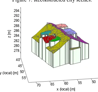
All the buildings in both datasets were reconstructed. Figure 7 a presents the reconsted city scene of Vaihingen, consisting of 21 buildings. Figure 7b presents the reconstructed Munich scene with 8 buildings.
3.3 Evaluation
The results of the reconstructed buildings are evaluated according to the evaluation of the the ISPRS benchmark project
(Rotten-0 20
(a) Side view of the reconstructed Vaihingen scene, wall segments (grey areas) are connecting the outer roof boundaries to ground or to other roof segments.
0
100 120 140 160
500
(b) Side view of the reconstructed Munich scene, wall segments (grey areas) are connecting the outer roof boundaries to ground or to other roof segments.
Figure 7. Reconstructed city scenes.
50
Figure 8. Detailed building model in a local coordinate system.
Tstep= 0.2 m, grid cell sizeC= 2.5 LiDAR points per cell,
resid-ual threshold R= 0.8 m. Segments from one height layer are separated by both, step edges and intersection edges.
steiner et al., 2012). The ground truth used by the ISPRS bench-mark project was not made available. Therefore, the results are evaluated against manually extracted 2D reference segment poly-gons. For the Vaihingen data set, ground truth was extracted from the ortho image delivered with the test data for the ISPRS bench-mark project. For the Munich data set, ground truth was extracted from high resolution ortho image. The following eight evaluation parameters are calculated:
• Completeness Cm =
T Pr
T Pr+F N
, where T Pr are true
positive andF Nare false negative reference polygons, whose area is≥2.5m2and which are overlapping by at least (T Pr
) or less than (F N) 50 % with estimated segment polygons.
Cm,10is computed analogously for segment areas≥10m2.
• CorrectnessCr =
T Pe
T Pe+F P
, whereT Pdare true
posi-tive andF P are false positive estimated segments, whose area is≥ 2.5m2 and which are overlapping by at least (T Pd) or less than (F P) 50 % with reference polygons.
Cr,10is computed analogously for segment areas≥10m2.
• RMSEcomputed from the 2D distancesdxyof the
esti-mated segment outline vertices to their reference segment, whiledxy>3m are neglected.
• NO: Number of oversegmented reference segments, i.e.
those corresponding to more than oneT Pd.
• NU: Number of undersegmenting estimated segsments, i.e.
those corresponding to more than oneT Pr.
• NC: Number of references which are both under- and
over-segmented.
3.4 Evaluation results
Tables 2 and 3 show the evaluation parameters for segmenta-tion. 2D segment outlines are evaluated against the reference segments. Results for the Vaihingen scene are compared to those of Awrangjeb and Fraser (2014), who apply the same evaluation method (section 3.3) to their segmentation results.
Method Cm(Cm,10) Cr(Cr,10)
Munich scene
proposed 80.4 (87.8) 98.6 (100.0)
Vaihingen scene
proposed 91.2 (95.0) 93.3 (97.3)
Awrangjeb & Fraser, 2014 76.4 (84.4) 83.3 (84.9)
Table 2. Completeness and correctness of the segmentation. Seg-mentation results of the Vaihingen Scene are compared to the re-sults of Awrangjeb and Fraser (2014).
Method NU NO NC RMSE
Munich scene
proposed 3 15 1 1.46
Vaihingen scene
proposed 8 25 0 0.56
Awrangjeb & Fraser, 2014 42 6 7 0.41
Table 3. Under- and oversegmentation and accuracy of the seg-mentation. Segmentation results of the Vaihingen Scene are com-pared to the results of Awrangjeb and Fraser (2014).
Tables 4 and 5 show the evaluation results for reconstruction. The outer boundaries of each group of adjacent roof triangles with equal segment label are projected to the x-y-plane and evaluated against the reference segments. Results for the Vaihingen scene are compared to those of the ISPRS benchmark project.
It has to be considered that the manually extracted ground truth might differ from the ground truth used by the ISPRS benchmark project.
4. DISCUSSION
The proposed method creates building models of high detail by triangulation. In contrast to triangulating the input LiDAR point cloud, adaptive 2.5D Dual Contouring has two main advantages:
Method Cm(Cm,10) Cr(Cr,10)
Munich scene
proposed 96.1 (100.0) 98.7 (100)
Vaihingen scene
proposed 100.0 (100.0) 95.4 (95.4)
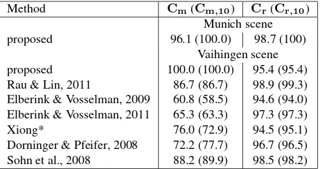
Rau & Lin, 2011 86.7 (86.7) 98.9 (99.3) Elberink & Vosselman, 2009 60.8 (58.5) 94.6 (94.0) Elberink & Vosselman, 2011 65.3 (63.3) 97.3 (97.3)
Xiong* 76.0 (72.9) 94.5 (95.1)
Dorninger & Pfeifer, 2008 72.2 (77.7) 96.7 (96.5) Sohn et al., 2008 88.2 (89.9) 98.5 (98.2)
Table 4. Completeness and correctness of the reconstruction. Re-sults of the Vaihingen Scene are compared to the reRe-sults of other methods (* see Rottensteiner et al., 2012).
Method NU NO NC RMSE
Munich scene
proposed 4 17 0 1.39
Vaihingen scene
proposed 13 32 1 0.72
Rau & Lin, 2011 36 10 3 0.66
Elberink & Vosselman, 2009 26 16 17 0.91 Elberink & Vosselman, 2011 38 0 3 0.94
Xiong* 40 2 2 0.84
Dorninger & Pfeifer, 2008 42 7 6 0.79
Sohn et al., 2008 36 5 14 0.75
Table 5. Under- and over-segmentation and accuracy of the re-construction. Results of the Vaihingen Scene are compared to the results of other methods (* see Rottensteiner et al., 2012).
Depending on the chosen level of detail (by setting the parame-tersCandR), points for building representation are reduced to a minimum at continuities. Second, step edges are always rep-resented as vertical walls, as vertices of a hyperpoint are always vertically arranged.
The novelty of the proposed reconstruction method is using a de-tailed segmentation as input to a 2.5D Dual Contouring approach. In contrast to Zhou and Neumann (2010), the proposed situation-adaptive QEF construction allows to model accurate step edges between segments from one height layer (Fig. 8). For each pair of local height layers within each grid cell, a decision is made whether to connect them either by an intersection edge or by a step edge. The step edge thresholdTstep, the residual for
quadtree collapsingR, and the grid cell sizeCare of equal im-portance for deciding whether a step edge or an intersection edge is locally created. IfCis chosen too high, roof segments which require both intersection edges and step edges to be modelled ac-curately (e.g. dormers) will only fall into one height layer and are “smoothed out”. The same smoothing effect happens ifRor
Tstepare chosen too high, or if roof segments within one roof
heigh layer are not segmented accurately, i.e. undersegmentation occurs (Fig. 9).
Zhou and Neumann (2010) do not carry out additional roof height layer segmentation. Consequnetly, no step edges can be created between parts of one height layer. In contrast, the presented adap-tive 2.5D Dual Contouring method can model superstructures such as dormers by allowing both intersection and step edges within one height layer.
A further advantage of the proposed method is that the building models’ level of detail can be influenced by changingCandR. Thereby, a trade-off between the desired level of detail on the one side, and the computation time and the number of hyperpoints in a building model on the other side has to be made. SmallerC
42 44 46 48 50 52 54 56 58
(a) Undersegmentation of the blue seg-ment. Opposite the dark green segment, a similar separate roof part should have been segmented.
(b) Reconstruction of a step edge between the blue and the dark green segment.
(c) Reconstruction, where no step edge can be modelled, because no different segments are identified.
Figure 9. Smoothed roof effect due to undersegmentation. If the roof height layer is undersegmented no step edges can be created, because only one local height layers is identified. However, the roof is approximated to fit the input point cloud in detail.
more roof triangles. However, if a regularized building model is required the large number of roof triangles increases the effort for postprocessing.
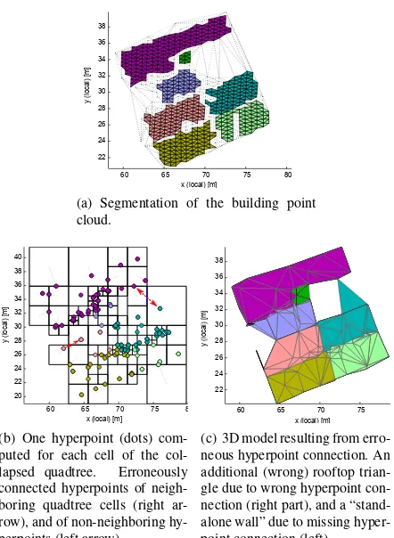
The building model’s 3D edges are constructed from connections of adjacent hyperpoints in the quadtree. In certain cases, this can lead to erroneous edges (Fig. 10b, right arrow). If hyperpoints from non-adjacent quadtree cells are connected to an edge, de-formations or “stand-alone walls” in the model can occur (Fig. 10b, left arrow).
5. CONCLUSION
A novel method for creating detailed building models with com-plex roof shapes from LiDAR point clouds is proposed in this paper. The 2.5D Dual Contouring method of Zhou and Neumann (2010) is used and adapted in a way that step edges and inter-section edges can be created between roof segments. A main contribution of this work is the modification and weighting of the Quadratic Error Function (QEF) for modeling step edges and intersection edges. The modeling depends on the step edge prob-abilities of local height layers. A prerequisite for adaptive 2.5D Dual Contouring is a roof segmentation technique which stops at smooth edges. The applied robust TIN-based region growing reli-ably stops at smooth edges. Consequently, undersegmentation is significantly reduced. The resulting building models show a very high fit to the input LiDAR points. Each roof segment is repre-sented by a triangulation, thus also non-planar roof shapes can be modelled. Subsequent model regularization is recommended, because buildings are represented by a large number of vertices. Errors in reconstruction result mostly from wrong or missing con-nections of the vertices. Thus, the way the concon-nections of the ver-tices to the building model should be more robust. Wrong con-nections could be avoided by checking for the consistency of the model with the building footprint. Under assumption that ing edges are mostly orthogonal or parallel to the main
build-60 65 70 75 80
(a) Segmentation of the building point cloud.
(b) One hyperpoint (dots) com-puted for each cell of the col-lapsed quadtree. Erroneously connected hyperpoints of neigh-boring quadtree cells (right ar-row), and of non-neighboring hy-perpoints (left arrow).
(c) 3D model resulting from erro-neous hyperpoint connection. An additional (wrong) rooftop trian-gle due to wrong hyperpoint con-nection (right part), and a “stand-alone wall” due to missing hyper-point connection (left).
Figure 10. Errors due to connectivity of hyperpoints from (non)-neighboring quadtree cells.
ing direction, the missing connections could be avoided by align-ing the buildalign-ing point cloud to the main buildalign-ing direction before the modeling procedure. The proposed workflow was tested and evaluated using two data sets with different characteristics and varying building complexity. Evaluation of the results has shown that both segmentation of LiDAR point clouds and reconstruction of buildings are comparable to the state-of-the-art methods.
ACKNOWLEDGEMENTS
The Vaihingen data set was provided by the German Society for Photogrammetry, Remote Sensing and Geoinformation (DGPF) Cramer (2010):
http://www.ifp.uni-stuttgart.de/dgpf/DKEP-Allg.html.
References
Awrangjeb, M. and Fraser, C. S., 2014. Automatic segmenta-tion of raw lidar data for extracsegmenta-tion of building roofs. Remote Sensing 6(5), pp. 3716–3751.
Brenner, C., 2000. Towards fully automatic generation of city models. International Archives of Photogrammetry, Remote Sensing and Spatial Information Sciences 33(B3/1), pp. 84– 92.
Brenner, C., 2005. Building reconstruction from images and laser scanning. International Journal of Applied Earth Observation and Geoinformation 6(3), pp. 187–198.
Cramer, M., 2010. The DGPF-test on digital airborne cam-era evaluationoverview and test design. Photogrammetrie-Fernerkundung-Geoinformation 2010(2), pp. 73–82.
Dorninger, P. and Pfeifer, N., 2008. A comprehensive automated 3D approach for building extraction, reconstruction, and regu-larization from airborne laser scanning point clouds. Sensors 8(11), pp. 7323–7343.
Fiocco, M., Bostrom, G., Gonalves, J. G. and Sequeira, V., 2005. Multisensor fusion for volumetric reconstruction of large out-door areas. In Proc. of the Fifth IEEE International Conference on 3-D Digital Imaging and Modeling 3DIM pp. 47–54.
Geibel, R. and Stilla, U., 2000. Segmentation of laser altimeter data for building reconstruction: different procedures and com-parison. International Archives of Photogrammetry, Remote Sensing and Spatial Information Sciences 33(B3/1), pp. 326– 334.
Haala, N. and Kada, M., 2010. An update on automatic 3D build-ing reconstruction. ISPRS Journal of Photogrammetry and Re-mote Sensing 65(6), pp. 570–580.
Kada, M. and McKinley, L., 2009. 3D building reconstruction from lidar based on a cell decomposition approach. Interna-tional Archives of Photogrammetry, Remote Sensing and Spa-tial Information Sciences 38(3), W4, pp. 47–52.
Kada, M. and Wichmann, A., 2012. Sub-surface growing and boundary generalization for 3D building reconstruction. IS-PRS Annals of the Photogrammetry, Remote Sensing and Spa-tial Information Sciences I-3, pp. 233–238.
Lafarge, F. and Mallet, C., 2012. Creating large-scale city mod-els from 3D-point clouds: A robust approach with hybrid rep-resentation. International Journal of Computer Vision 99(1), pp. 69–85.
Maas, H. G. and Vosselman, G., 1999. Two algorithms for ex-tracting building models from raw laser altimetry data. IS-PRS Journal of Photogrammetry and Remote Sensing 54(2), pp. 153–163.
Matei, B. C., Sawhney, H. S., Samarasekera, S., Kim, J. and Ku-mar, R., 2008. Building segmentation for densely built urban regions using aerial lidar data. In Proc. of the IEEE Conference on Computer Vision and Pattern Recognition (CVPR) pp. 1–8.
Meng, X., Currit, N. and Zhao, K., 2010. Ground filtering al-gorithms for airborne lidar data: A review of critical issues. Remote Sensing 2(3), pp. 833–860.
Nurunnabi, A., Belton, D. and West, G., 2012. Robust segmen-tation in laser scanning 3D point cloud data. In Proc. of the IEEE International Conference on Digital Image Computing Techniques and Applications (DICTA) 1, pp. 1–8.
Oude Elberink, S. and Vosselman, G., 2009. Building reconstruc-tion by target based graph matching on incomplete laser data: analysis and limitations. Sensors 9(8), pp. 6101–6118.
Perera, S. N., Nalani, H. A. and Maas, H. G., 2012. An automated method for 3D roof outline generation and regularization in airbone laser scanner data. ISPRS Annals of the Photogram-metry, Remote Sensing and Spatial Information Sciences I-3, pp. 281–286.
Rau, J. Y. and Lin, B. C., 2011. Automatic roof model reconstruc-tion from als data and 2d ground plans based on side projecreconstruc-tion and the tmr algorithm. ISPRS Journal of Photogrammetry and Remote Sensing 66(6), pp. 13–27.
Rottensteiner, F., 2003. Automatic generation of high-quality building models from lidar data. IEEE Computer Graphics and Applications 23, pp. 42–50.
Rottensteiner, F., Sohn, G., Jung, J., Gerke, M., Baillard, C., Ben-itez, S. and Breitkopf, U., 2012. The ISPRS benchmark on urban object classification and 3D building reconstruction. IS-PRS Annals of Photogrammetry, Remote Sensing and Spatial Information Sciences I-3, pp. 293–298.
Sampath, A. and Shan, J., 2007. Building boundary tracing and regularization from airborne lidar point clouds. Photogram-metric Engineering and Remote Sensing 73(7), pp. 805–812.
Sampath, A. and Shan, J., 2010. Segmentation and reconstruc-tion of polyhedral building roofs from aerial lidar point clouds. IEEE Transactions on Geoscience and Remote Sensing 48(3), pp. 1554–1567.
Sohn, G., Huang, X. and Tao, V., 2008. Using a binary space partitioning tree for reconstructing polyhedral building models from airborne lidar data. Photogrammetric Engineering and Remote Sensing 74(11), pp. 1425–1438.
Sohn, G., Jwa, Y., Jung, J. and Kim, H., 2012. An implicit reg-ularization for 3D building rooftop modeling using airborne lidar data. ISPRS Annals of Photogrammetry, Remote Sensing and Spatial Information Sciences I-3, pp. 305–310.
Sun, S. and Salvaggio, C., 2013. Aerial 3D building detection and modeling from airborne lidar point clouds. IEEE Journal of Selected Topics in Applied Earth Observations and Remote Sensing 6(3), pp. 1440–1449.
Tarsha-Kurdi, F., Landes, T. and Grussenmeyer, P., 2008. Ex-tended ransac algorithm for automatic detection of building roof planes from lidar data. The photogrammetric journal of Finland 21(1), pp. 97–109.
Verma, V., Kumar, R. and Hsu, S., 2006. 3D building detec-tion and modeling from aerial lidar data. In Proc. of the IEEE Computer Society Conference on Computer Vision and Pattern Recognition 2, pp. 2213–2220.
Vosselman, G. and Dijkman, S., 2001. 3D building model recon-struction from point clouds and ground plans. International Archives of Photogrammetry Remote Sensing and Spatial In-formation Sciences 34(3/W4), pp. 37–44.
Vosselman, G., Gorte, B. G., Sithole, G. and Rabbani, T., 2004. Recognising structure in laser scanner point clouds. Interna-tional Archives of Photogrammetry Remote Sensing and Spa-tialInformation Sciences 46(8), pp. 33–38.
Wang, J. and Shan, J., 2009. Segmentation of lidar point clouds for building extraction. In Proc. of the Annual Conference of the American Society for Photogrammetry and Remote Sens-ing pp. 9–13.
Wang, R., 2013. 3D building modeling using images and lidar: a review. International Journal of Image and Data Fusion 4(4), pp. 273–292.
Zhang, W., Chen, Y., Yan, K., Yan, G. and Zhou, G., 2012. Primitive-based 3D building reconstruction method tested by reference airborne data. International Archives of the Pho-togrammetry, Remote Sensing and Spatial Information Sci-ences 39(B3), pp. 373–378.
Zhou, Q. Y. and Neumann, U., 2008. Fast and extensible building modeling from airborne lidar data. In Proc. of the 16th Inter-national Conference on Advances in Geographic Information Systems, ACM GIS 2008 (on CD-ROM).