A SPATIO-TEMPORAL FRAMEWORK FOR MODELING ACTIVE LAYER THICKNESS
J. Touyza, D. A. Streletskiyb, F. E. Nelsonc, T. V. Apanasovicha
aDept. of Statistics, The George Washington University, Washington, DC, 20052 USA-(joshuahtouyz, apanasovich)@gwu.edu b
Dept. of Geography, The George Washington University, Washington, DC, 20052 USA - [email protected] c
Dept. of Earth, Environmental, and Geographical Sciences, Northern Michigan University, Marquette, MI 49855 USA
KEY WORDS:Spatio-temporal Statistics, Active Layer Thickness, Covariance Functions, Geostatistics, Circumpolar Active Layer Monitoring, Cryosphere
ABSTRACT:
The Arctic is experiencing an unprecedented rate of environmental and climate change. The active layer (the uppermost layer of soil between the atmosphere and permafrost that freezes in winter and thaws in summer) is sensitive to both climatic and environmental changes, and plays an important role in the functioning, planning, and economic activities of Arctic human and natural ecosystems. This study develops a methodology for modeling and estimating spatial-temporal variations in active layer thickness (ALT) using data from several sites of the Circumpolar Active Layer Monitoring network, and demonstrates its use in spatial-temporal interpolation. The simplest model’s stochastic component exhibits no spatial or spatio-temporal dependency and is referred to as the na¨ıve model, against which we evaluate the performance of the other models, which assume that the stochastic component exhibits either spatial or spatio-temporal dependency. The methods used to fit the models are then discussed, along with point forecasting. We compare the predicted fit of the various models at key study sites located in the North Slope of Alaska and demonstrate the advantages of space-time models through a series of error statistics such as mean squared error, mean absolute and percent deviance from observed data. We find the difference in performance between the spatio-temporal and remaining models is significant for all three error statistics. The best stochastic spatio-temporal model increases predictive accuracy, compared to the na¨ıve model, of 33.3%, 36.2% and 32.5% on average across the three error metrics at the key sites for a one-year hold out period.
1. INTRODUCTION AND BACKGROUND
The Arctic is experiencing an unprecedented rate of environmen-tal and climate change (Hinzman et al., 2005). Vast areas of the Arctic are underlain by permafrost, defined as earth materials that remain at or below0◦Ccontinuously for two or more years. The permafrost regions occupy nearly a quarter of the Earth’s terres-trial surface (Zhang et al., 1999).
The active layer is the uppermost layer of soil or other earth ma-terial above permafrost that experiences seasonal freezing and thawing. The thickness of the active layer (ALT) plays an im-portant role in the ecology, hydrology and geomorphology of cold environments. Knowledge about the spatial-temporal vari-ability of ALT is crucial for engineering applications and con-struction in northern regions (Streletskiy et al., 2012). Permafrost degradation reported in the Arctic has the potential to influence the balance of greenhouse gases and may pose significant haz-ards to local infrastructure, especially in permafrost ice-rich areas where extensive landscape changes result in subsidence and the development of irregular surfaces over extensive areas, known as thermokarst terrain (Streletskiy et al., 2015). Consequently, un-derstanding the dynamics that contribute to shifts in ALT is of interest at both local and global scales.
The thickness of the active layer varies from centimeters to sev-eral meters along the latitudinal bioclimatic gradient, and is present everywhere where there is permafrost. Its calculation is often ap-proximated analytically using the Stefan Solution e.g., (Jumikis, 1978), given in one of its most basic forms by:
X=
s
2λs(nDDT)
ρwL (1)
whereX is the annual depth of thaw (m),λis the thermal
con-ductivity of the substrate (W/m◦C), DDT is the degrees days of thaw, a time-temperature integral representing cumulative sum-mer warmth at the surface (◦C days),sis a scale factor (s/day), ρis the dry density of the substrate (kg/m3),wis water content expressed as a proportion of dry weight, andLis the latent heat of fusion (J/kg).
Calculation of ALT over extensive areas is a challenging under-taking owing to the high variability and unavailability of detailed subsurface information. Accordingly, many studies have assumed that subsurface characteristics are constant over geographic space, and used even more simplified versions of the Stefan relation. Compounding this situation is the fact that few spatial time series of active-layer thickness (ALT) existed prior to about 1990. For this reason, the Circumpolar Active Layer Monitoring (CALM) program was implemented in the 1990s. The CALM program maintains a network of more than 250 permafrost observatories that monitor active layer and near-surface permafrost responses to climate change over multi-decadal time scales. CALM has pro-duced a large number of publications, many of which address spa-tial time series using relatively simple statistical strategies (Shik-lomanov et al., 2012).
dynam-ics of ALT. Process-oriented analytical and numerical models, of varying complexity, have been developed to explain changes in ALT. Similarly, several statistical procedures have been used to map and analyze the spatial variability of ALT, including re-gression modeling (Nelson et al., 1997), kriging (Shiklomanov and Nelson, 2003), nested sampling and analysis (Nelson et al., 1999), and spatial autocorrelation analysis (Nelson et al., 1998). Some of this literature has been summarized in (Brown et al., 2000), (Nelson et al., 2008), and (Mishra et al., 2013) , and a comparative study of various models was published by (Shiklo-manov et al., 2007). However, the literature concerned with mod-eling space-time variability using continuous parameters (Qian and Apanasovich, 2014) is small. This study is concerned with developing a methodological framework for modeling ALT us-ing Gaussian random fields with non-separable space-time co-variance structures. The primary points addressed are: (a) data availability at eight site locations in northern Alaska; (b) theory about spatial-temporal covariance structures; (c) specification of stochastic spatial and spatio-temporal models; (d) introduction of four geostatistical ALT models formulated as the sum of a deter-ministic trend and a stochastic component; (e) differentiation be-tween the models, based on specification of their stochastic com-ponents.
2. DATA AVAILABILITY
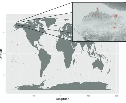
The data used to model ALT were drawn from the CALM database. CALM data are available publicly, and can be accessed online at the CALM website (www.gwu.edu/∼calm). Eight sites located in the North Slope of Alaska were selected to develop the model. The sites were selected based on data availability and proxim-ity to settlements in hope that the developed methodology can be used for societal benefits in these settlements. Basic infor-mation about the sites is shown in 1. These sites were selected for analysis because of the availability of high-quality data, their contrasting topography, and their proximity to indigenous popu-lations (Barrow, Atkasuk), a major operating oil field (West Dock - Purdhoe Bay), and environmental organizations (University of Alaska’s Toolik Lake Long-Term Ecological Research station). These characteristics impart social, commercial, and educational relevance.
Active layer data were obtained at different scales, according to one of two schemes, both employing a systematic spatial sam-pling protocol. Under the first scheme an11×11grid of 121 stations was sampled over 100 m increments to form a 1×1 km square array. In the second scheme data were sampled over a 100×100 m square array with stakes separated every 10 m. Data are recorded annually by manual probing during late August or early September, when ALT is near its maximum annual value. For computational purposes, the working assumption was made that measurements occur at precisely annual intervals, so that modeling procedures can be implemented using regular intervals.
Table 1 summarizes data availability and characteristics of the de-sign. Although data are available at most sites between the years 1995-2014, there are missing values. This may be by design, for example, at point locations with rocky substrates that do not permit manual probing. Two sampling grids that contain a rela-tively large number of such points are Imnavait Creek and Toolik Lake. Accordingly, their sample design contains 49 and 74 sta-tions, respectively. These are very sparse in comparison with the remaining site locations, which each have at least 99 stations at which ALT can be measured. For succinctness, we use site codes to reference sampling locations in the remainder of this paper.
During exploratory data analysis, ALT was compared spatially and cross-temporally. ALT points that vary substantially from
Longitude
La
ti
tu
d
e
Figure 1. Site Locations
others may be an artifact of terrain characteristics or the result of an unseasonably warm summer. For example, the U1 site is bisected by a gravel-rich beach-ridge, for which readings in that sampling locale are significantly higher than neighboring val-ues. Using Anselin’s local Moran I statistic (Anselin, 1995), ALT readings that are significantly different from their neighbors were identified and removed.
3. MODEL
3.1 Geostatistical Modelling
Geophysical processes are variable over both space and time. Geostatistical approaches typically model continuous spatio-temporal observations by the sum of a systematic trend and stochastic com-ponents:
X(s, t) =m(s, t)+ξ(s, t)+Z(s, t), s∈ S ⊆Rd, t∈ T ⊆R, (2) wherem(s, t) =E{X(s, t)}, the mean function or global trend, is smooth and deterministic,ξ(s, t)is a Gaussian field of spatially and temporally uncorrelated mean zero errors, andZ(s, t)is a mean-zero Gaussian random function. The error processξ(s, t) has covariance function:
Cov{ξ(s, t), ξ(s+h, t+u)}=
(
τ2
h= 0, u= 0 0 h6= 0, u6= 0 (3) whereasZ(s, t)is fully characterized by its covariance function and explains space-time variability not captured by the mean func-tion or error process i.e. the microscale variafunc-tion. The covariance function ofX(s, t)is defined as:
CX{(s,s+h),(t, t+u)}:=Cov{X(s, t), X(s+h, t+u);θ}, (4)
wheres,s+h∈ S;t, t+u∈ T,θ∈ΘandΘis the parameter space. In general, some assumptions were made with respect to the stochastic space-time processZ(s, t). Two common working assumptions are isotropy and separability. When the data support the two assumptions, model complexity and computational inten-sity are reduced.
In the context of covariance functions, whenZ(s, t)is both trans-lation and rotation invariant, it is said to beisotropic:
where|| · ||is the Euclidean distance.
A processZ(s, t)is said to beseparableif the covariance func-tion can be factored into purely spatial and temporal components:
Cov{Z(s, t), Z(s+h, t+u)}=CS{s,s+h}CT{t, t+u} (6) wheres+h∈ Sandt+u∈ T. Separable models do not allow for space-time interaction and consequently do not adequately model physical processes when interaction is present. Accord-ingly, non-separable models generally have better predictive per-formance than separable models. WhenZ(s, t)is isotropic and separable its covariance function can be written as:
Cov{Z(s, t), Z(s+h, t+u)}=CS{||h||}CT{|u|} (7) whereh∈Rdandu∈R.
3.2 Stochastic Spatial and Spatio-Temporal Models
We consider two spatial covariance functionsCS{||h||}. The first is the Mat´ern covariance:
CS{h;θ}= σ of the second kind. The Mat´ern is selected due to its flexibility modeling different degrees of smoothness. A second commonly used spatial covariance function is the powered-exponential co-variance, which has a closed parametric form and does not rely on the Bessel function, easing subsequent parameter estimation:
CS{h;θ}=σ2exp
A popular choice for expressing temporal dependency is the gen-eralized Cauchy covariance function (Gneiting et al., 2006):
CT{u;θ}= σ poral processes can be combined through the separable model. When the spatial process’s covariance is Mat´ern and the tempo-ral process’s covariance matrix is Cauchy the resulting separable function is proportional to the product of the covariances:
Cov{h, u;θ}= σ separable space-time process obtains when the spatial process’s covariance matrix is a powered exponential whereas the temporal process follows a Cauchy:
A non-separable space-time version of equation (12) used in the literature (Gneiting et al., 2006), because of its tractability, is Gneiting’s powered exponential-Cauchy model with covariance
function:
>0. The parameterβcontrols space-time interaction and whenβ = 0the covariance function is proportional to the separable model. Similarly, forγ = 0, Z(s, t) reduces to a temporal process with Cauchy covariance (CT) whereas whenδ = 0,Z(s, t)reduces to a purely spatial process with powered-exponential covariance (CS).
3.3 Modeling Active Layer Thickness
Four models are considered. The first, na¨ıve, model assumes no stochastic spatio-temporal variability,Z(s, t), so that:
X(s, t) =m(s, t) +ξ(s, t), s∈ S, t∈ T. (14) wherem(s, t)is the mean function andξ(s, t)is the error pro-cess. The spatial and temporal trends do not interact so the mean function is defined as the sum of spatial and temporal trends:
m(s, t) =mS(s;υ) +mT(t;λ), (15)
whereυ = {υi}i∈I,λ = {λj}j∈J are unknown parameters with index setsI,J and the functionsmS(s;υ)andmT(t;λ) are known up to the value of their parameters .
When there are a small number of parameters, as in polynomial regression, the microscale variation is not captured by the mean function hence it is not flexible enough to capture all space-time variation. Accordingly, we add a stochastic component to ac-count for the microscale variation. The remaining models include a global trend and stochastic space-time component:
X(s, t) =m(s, t) +ξ(s, t) +Z(s, t), s∈ S, t∈ T (16) wherem(s, t), ξ(s, t)andZ(s, t)were previously defined. It is possible that microscale variation occurs only in space and here we consider the reduced model. For a fixedt ∈ T, Model 2’s covariance does not depend on time and is given by:
Cov{Z(s, t), Z(s+h, t+u)}=
(
CS{||h||} u= 0 0 u6= 0. (17) WhenZ(s, t)’s microscale variation is both in space and time, we refer to it as Model 3, whereas when it is non-separable it is referred to as Model 4.
3.4 Fitting Models to Data
Following the convention of (Zimmerman and Michael, 2010), we assume the na¨ıve model’s spatial trend is modeled by at most, a second order polynomial:
their corresponding unknown parameters. We assume the tem-poral trend follows, at most, a second order polynomial equation with Fourier frequencycos(ωt):
mT(t;λ) =λ0+λ1cos(ω(t+λ2)) +λ3t+λ4t 2
wheret∈ T ⊆Rand{λi}4
i=0are the corresponding unknown
parameters. The parameters of the spatial and temporal trends are estimated using non-linear least squares.
With respect to models 2-4, once the global trend is fit, the param-eters of the covariance function of the residualsZ(s, t)(CZ(·,·;θ)) are estimated. When maximum likelihood criteria are used, ex-act schemes rely on repeated formation and inversion of the co-variance matrix and evaluation of its determinant which can be computationally demanding. Rather, composite likelihood, an approximate likelihood method, is used to estimate the covari-ance parameters. Using composite likelihood, a pseudolikelihood function is constructed from the marginal densities of all pair-wise differences among the observations and maximized. Using a spatio-temporal version of the scheme proposed by (Curriero and Lele, 1999), we find the parametersθ∈Θthat maximize the spatio-temporal composite likelihood function:
wherenis the number of observations,z(ˆsi, ti)is the value of the residual at locationsiand timeti,θ∈ΘZ⊆Θand
CZ{si−sj, ti−tj;θ}:=Cov{Z(si, ti), Z(sj, tj);θ}. (22) Models are fit inRusing theCompRandFldpackage (Padoan and Bevilacqua, 2015).
3.5 Prediction
For separable and non-separable spatio-temporal models the sim-ple point forecast at locations0 ∈ Sand timet0 ∈ T is given where ci0 is the vector of covariances between the residuals,
(ˆz(s,t) ={z(ˆsi, tj)}i,j∈S,T)and predicted variables(z(s0, t0) = {z(si, t0)}i∈S),CZis the variance-covariance matrix ofZ(s, t) andz(ˆs, t)is the vector of residuals.
The predicted value for Model 1 at locationss0 ∈ S and time
t0∈ T is similarly given by:
ˆ
µ(s0, t0) = ˆm(s0, t0) (24)
which is the global trend predicted at valuess0andt0.
4. MODEL COMPARISON
4.1 Model Comparison Test
In the absence of temporal correlation the spatio-temporal mod-els, Model 3 and Model 4, reduce to the stochastic spatial model, Model 2, with Mat´ern and powered exponential covariances, re-spectively. Model 2 has four estimable parameters whereas Model 3 has seven and Model 4 has eight. We compare the fitted nested spatial models and saturated spatio-temporal models to one an-other at the eight sites using likelihood ratio tests. We test whether there is a significant difference between spatial Mat´ern and spatio-temporal Mat´ern-Cauchy models as well as the spatial powered exponential and spatio-temporal powered exponential-Cauchy mod-els.
4.2 Time-Forward Prediction
To assess the predictive performance of increasingly complex models we use time-forward predictions of the ALT during the
test period based on fitted models in the training period. In par-ticular, one-year ahead spatio-temporal predictions for ALT mea-sures are made at each of the stations for the four models. A one-year hold out set, the year 2014, was used to rank model fits based on several metrics. Predicted root mean squared er-ror (PRMSE), predicted mean absolute erer-ror (PMAE) and pre-dicted mean percentage difference (PMPD) were used to assess the quality of point forecasts. For yeart0 ∈ T and sitess0 ∈ S
the prediction metrics are defined as:
P RM SE=
hold out set and|S|is the cardinality ofS.
5. RESULTS AND DISCUSSION
The methodological framework elaborated above was applied to the ALT grids summarized in Table 1. We first applied the likeli-hood ratio test to spatial and spatio-temporal models to assess fit. Table 2 lists the log-likelihood for Models 2-4. Since allp-values are close to zero the likelihood ratio tests indicate a significant difference in model fit (p≈0) between spatio-temporal models and their spatial counterparts for each of the eight sites.
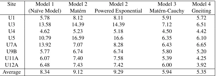
We subsequently compared models based on the time-forward error measures at the various sites. Tables 3-5 list the PRMSE, PRMAE and PMPD of Models 1-4 for a one-year time forward period; Table 6 summarizes the relative difference in performance of the non-separable model to the other three.
The spatio-temporal models time-forward errors are lower than in deterministic and spatial stochastic models at seven of the eight sites. In particular, for all sites except at site U7A the non-separable model has the lowest PRMSE, PMAE and PMPD.
Using a paired Wilcoxon non-parametric permutation test with exactp-values we assessed whether systematic differences in pre-dictive performance between sites existed for Models 3 and 4. The test indicated the PRMSE, PMAE and PMPD for the Model 3 and Model 4 were not statistically significant as thep-values for the PRMSE, PMAE, and PMPD were allp >0.05. In contrast, the test indicated a significant difference between spatio-temporal models and Models 1 and 2. Their p-values are summarized in Tables 7-8.
models averages time-forward predictions across the eight sites are within 19.3%, 20.0% and 20.4% of the true values. The non-separable spatio-temporal model’s average PRMSE, PMAE and PMPD across the eight sites are identified as the smallest among the models. Relative to the na¨ıve model, the increase in aver-age predictive accuracy across the eight sites for the three error metrics is 33.3%, 36.2% and 32.5%.
Second, when spatio-temporal interaction is present, predictive performance may increase. Table 9 lists the values of the interac-tion parameterβfor the eight sites. At sites U3, U11A and U12A, where spatio-temporal interaction is present, there are predictive performance gains for the non-separable spatio-temporal model relative to the separable spatio-temporal model. The most notice-able decrease in predictive errors occur at sites U11A and U12A, where the landscapes are homogeneous and the spatio-temporal interaction is detectable. The relative decrease of the PRMSE, PMAE and PMPD of the non-separable model to the separable model are by 20.6%, 27.9% and 28.7%, respectively.
6. CONCLUSIONS
This study introduces a methodological framework for modeling ALT, using four models that are the sum of a systematic trend and stochastic component. The na¨ıve model, against which we com-pare the other models, assumes ALT is completely determined by the global trend, whereas the other models characterize mi-croscale variability through either spatial or spatio-temporal de-pendency. We assessed the models’ predictive accuracy at eight sites which possess different degrees of sparsity for a one-year forward period using root mean squared error, mean absolute er-ror, and mean performance difference.
The spatio-temporal models significantly reduce the time-forward errors metrics when compared to both deterministic and spatial stochastic models. The temporal stochastic component subse-quently plays a role characterizing active layer thickness dynam-ics and decreasing prediction point errors.
Despite grid sparsity the spatio-temporal model was able to cap-ture the residual variability through its temporal component, and generate predictions superior to those of the deterministic and spatially stochastic models. The implication for researchers is that complete grids may not be necessary to characterize ALT dynamics, possibly resulting in decreased setup and operational costs. When landscapes are homogeneous and interaction is de-tectable measurement error is further reduced.
The largest limitation in the current approach is that a non-separable Gneiting Cauchy-Mat´ern could not be implemented in the analy-sis given the limitations of the packageCompRandFld. Had the option for a non-separable Gneiting Cauchy-Mat´ern been avail-able the analysis would have allowed comparison of nested spa-tial, separable and non-separable models.
A future route of research is to develop a full stochastic model that considers not only ALT, but other variables such as tempera-ture, snow coverage, relative humidity and solar radiation across space simultaneously. Some of the multivariate spatial models currently of interest in the statistics community may also be use-ful to this end (Apanasovich and Genton, 2010, Apanasovich et al., 2012).
ACKNOWLEDGEMENTS
This work is part of the thesis of the first author. We thank GWU UFF for promoting cross-disciplinary collaboration resulting in the advancement of the publication. This publication was sup-ported by NSF grants ARC-1204110, PLR-1534377, and RSF project 14-17-00037.
REFERENCES
Anselin, L., 1995. Local indicators of spatial associationLISA. Geographical analysis 27(2), pp. 93–115.
Apanasovich, T. V. and Genton, M. G., 2010. Cross-covariance functions for multivariate random fields based on latent dimen-sions. Biometrika 97(1), pp. 15–30.
Apanasovich, T. V., Genton, M. G. and Sun, Y., 2012. A valid Mat´ern class of cross-covariance functions for multivariate ran-dom fields with any number of components. Journal of the Amer-ican Statistical Association 107(497), pp. 180–193.
Biskaborn, B., Lanckman, J.-P., Lantuit, H., Elger, K., Strelet-skiy, D., Cable, W. and Romanovsky, V., 2015. The Global Ter-restrial Network for Permafrost Database: metadata statistics and prospective analysis on future permafrost temperature and active layer depth monitoring site distribution. Earth System Science Data Discussions 8(1), pp. 279–315.
Brown, J., Hinkel, K. and Nelson, F., 2000. The Circumpolar Ac-tive Layer Monitoring (CALM) program: historical perspecAc-tives and initial results. Polar Geography 24(3), pp. 166–258.
Curriero, F. C. and Lele, S., 1999. A composite likelihood ap-proach to semivariogram estimation. Journal of Agricultural, Bi-ological, and Environmental statistics pp. 9–28.
Gneiting, T., Genton, M. G. and Guttorp, P., 2006. Geostatistical space-time models, stationarity, separability, and full symmetry.
Hinzman, L. D., Bettez, N. D., Bolton, W. R., Chapin, F. S., Dyurgerov, M. B., Fastie, C. L., Griffith, B., Hollister, R. D., Hope, A., Huntington, H. P. et al., 2005. Evidence and implica-tions of recent climate change in northern Alaska and other Arctic regions. Climatic Change 72(3), pp. 251–298.
Jumikis, A. R., 1978. Thermal geotechnics.
Mishra, U., Jastrow, J., Matamala, R., Hugelius, G., Ping, C. and Michaelson, G., 2013. Spatial variability of surface organic hori-zon thickness across Alaska. In: AGU Fall Meeting Abstracts, Vol. 1, p. 03.
Nelson, F., Hinkel, K., Shiklomanov, N., Mueller, G., Miller, L. and Walker, D., 1998. Active-layer thickness in north-central Alaska: systematic sampling, scale, and spatial autocorrelation. Journal of Geophysical Research: Atmospheres (1984–2012) 103(D22), pp. 28963–28973.
Nelson, F., Shiklomanov, N. and Mueller, G., 1999. Variability of active-layer thickness at multiple spatial scales, north-central Alaska, U.S.A. Arctic, Antarctic, and Alpine Research pp. 179– 186.
Nelson, F., Shiklomanov, N., Hinkel, K. and Brown, J., 2008. Decadal results from the Circumpolar Active Layer Monitoring (CALM) program. In: Proceedings of the Ninth International Conference on Permafrost, Fairbanks, Alaska, June, pp. 1273– 1280.
Nelson, F., Shiklomanov, N., Mueller, G., Hinkel, K., Walker, D. and Bockheim, J., 1997. Estimating active-layer thickness over a large region: Kuparuk River basin, Alaska, U.S.A. Arctic and Alpine Research pp. 367–378.
Qian, C. and Apanasovich, T. V., 2014. Spatial-temporal mod-eling of active layer thickness. SIAM Undergraduate Research Online.
Schaefer, K., Lantuit, H., Romanovsky, V., Schuur, E. and G¨artner-Roer, I., 2012. Policy implications of warming per-mafrost.
Shiklomanov, N. and Nelson, F., 2003. Statistical representation of landscape-specific active-layer variability. In: Proceedings of the Eighth International Conference on Permafrost, Zurich, Switzerland. AA Balkema: Lisse, pp. 21–25.
Shiklomanov, N. I., Anisimov, O. A., Zhang, T., Marchenko, S., Nelson, F. E. and Oelke, C., 2007. Comparison of model-produced active layer fields: Results for northern Alaska. Journal of Geophysical Research: Earth Surface (2003–2012).
Shiklomanov, N. I., Streletskiy, D. A. and Nelson, F. E., 2012. Northern Hemisphere Component of the Global Circumpolar Ac-tive Layer Monitoring (CALM) Program. In: Proceedings of the Tenth International Conference on Permafrost, Salekhard, Yamal-Nenets Autonomous District, Russia, pp. 25–29.
Streletskiy, D. A., Shiklomanov, N. I. and Nelson, F. E., 2012. Permafrost, infrastructure and climate change: A GIS-based landscape approach to geotechnical modeling. Arctic, Antarctic, and Alpine Research 44(3), pp. 368–380.
Streletskiy, D., Anisimov, O. and Vasiliev, A., 2015. Chapter 10 - Permafrost Degradation. In: W. Haeberli, C. Whiteman and J. F. Shroder (eds), Snow and Ice-Related Hazards, Risks and Disasters, Academic Press, Boston, pp. 303 – 344.
Zhang, T., Barry, R. G., Knowles, K., Heginbottom, J. and Brown, J., 1999. Statistics and characteristics of permafrost and ground ice distribution in the Northern Hemisphere. Polar Geog-raphy 23(2), pp. 132–154.
Zimmerman, D. L. and Michael, S., 2010. Handbook of Spatial Statistics. CRC Press, chapter Classical Geostatistical Methods.
Site Name Site Code Years Sampling Design Coordinates # Measurements
Barrow U1 20 1×1 km 71◦19’N, 156◦36’W 116
Atkasuk U3 20 1×1 km 70◦27’N, 157◦24’W 102
West Dock U4 19 100×100m 70◦22’N, 148◦33’W 121
West Dock U5 19 1×1km 70◦22’N, 148◦33’W 103
Betty Pingo U7A 19 1×1 km 70◦17’N, 148◦52’W 99
Happy Valley U9B 19 100×100 m 69◦10’N, 148◦50’W 112
Imnavait Creek U11A 20 1×1 km 68◦30’N, 149◦30’W 49
Toolik U12A 20 1×1 km 68◦37’N, 149◦36’W 74
Table 1. Site Locations and Features
Site Model 2 Model 3 Model 3 Model 4
Mat´ern Mat´ern-Cauchy Powered Exponential Gneiting
U1 -6024376 -6018046 -5589312 -5585464
U3 -6884152 -6860606 -7045597 -6860593
U4 -8784495 -8766294 -6555215 -6553003
U5 -11149585 -10813754 -14623955 -11377347
U7A -6881255 -6881216 -6894816 -6881192
U9B -7240268 -7227548 -7122015 -7108969
U11A -1929512 -1926401 -1927920 -1926425
U12A -1157276 -1073743 -1261506 -1095846
Table 2. Log-likelihood of Models 2-4
Site Model 1 Model 2 Model 2 Model 3 Model 4
(Na¨ıve Model) Mat´ern Powered Exponential Mat´ern-Cauchy Gneiting
U1 8.36 8.28 8.26 6.98 6.79
U3 19.98 18.78 18.78 11.20 10.80
U4 6.17 6.82 6.76 6.01 5.94
U5 13.10 16.38 16.4 7.97 7.61
U7A 16.45 8.82 9.68 7.83 8.05
U9b 7.14 8.28 8.29 7.19 6.67
U11A 7.92 9.63 9.85 6.74 5.64
U12A 8.70 10.04 10.05 8.30 6.23
Average 10.81 11.07 11.20 7.78 7.22
Table 3. PRMSE for Models 1-4
Site Model 1 Model 2 Model 2 Model 3 Model 4
(Na¨ıve Model) Mat´ern Powered Exponential Mat´ern-Cauchy Gneiting
U1 5.78 8.12 8.11 5.91 5.72
U3 13.58 14.39 14.39 7.12 6.51
U4 4.62 5.23 5.18 4.50 4.42
U5 10.79 16.59 16.6 6.35 6.10
U7A 13.92 7.07 8.28 6.43 6.65
U9B 5.77 6.74 6.74 5.80 5.20
U11A 6.07 7.40 7.58 5.39 4.25
U12A 6.48 7.43 7.42 6.00 3.92
Average 8.34 9.12 9.29 5.94 5.35
Site Model 1 Model 2 Model 2 Model 3 Model 4 (Na¨ıve Model) Mat´ern Powered Exponential Mat´ern-Cauchy Gneiting
U1 20.2% 22.9% 22.9% 20.1% 19.4%
U3 23.7% 28.4% 28.4% 13.4% 12.5%
U4 14.2% 16.4% 16.3% 14.2% 13.9%
U5 24.7% 30.1% 30.1% 13.8% 13.6%
U7A 32.3% 16.1% 18.7% 14.7% 15.3%
U9B 14.0% 16.3% 16.3% 14.2% 13.0%
U11A 12.5% 15.3% 15.7% 11.5% 9.0%
U12A 12.6% 14.5% 14.5% 11.5% 7.4%
Average 19.3% 20.0% 20.4% 14.2% 13.0%
Table 5. PMPD for Models 1-4
Site Model 1 Model 2 Model 2 Model 3
(Na¨ıve Model) Mat´ern Powered Exponential Mat´ern-Cauchy
PRMSE 33.3% 33.1% 35.6% 7.22%
PMAE 36.2% 41.4% 42.4% 9.96%
PMPD 32.5% 34.9% 36.1% 8.20%
Table 6. Average Performance of Models 1-3 to Model 4
Metric Model 1 Model 2 Model 2
(Na¨ıve Model) Mat´ern Powered Exponential
PRMSE 0.0078 0.027 0.027
PMAE 0.0039 0.0039 0.0039
PMPD 0.0039 0.0039 0.0039
Table 7. Model 3 -p-values for paired Wilcoxon test
Metric Model 1 Model 2 Model 2
(Na¨ıve Model) Mat´ern Powered Exponential
PRMSE 0.0039 0.0039 0.0039
PMAE 0.0039 0.0039 0.039
PMPD 0.0039 0.0039 0.039
Table 8. Model 4 -p-values for paired Wilcoxon test
Site U1 U3 U4 U5 U7A U9B U11A 12A
Interaction parameter 0.00 0.05 0.00 0.00 0.00 0.00 1.00 1.00