ASSESSMENT OF ICE-DAM COLLAPSE BY TIME-LAPSE PHOTOS
AT THE PERITO MORENO GLACIER, ARGENTINA
Lenzano, M. G.a, *, Lannutti, E.b, Toth , C.c, Lenzano, L.b, Lovecchio, A.b
a
Universidad Nacional de Cuyo-CONICET, Mendoza, Argentina – [email protected] b
Depto. de Geomática. IANIGLA-CCT, CONICET, Mendoza, Argentina – (elannutti, llenzano, anlovecchio)@mendoza-conicet.gob.ar
c
Department of Civil, Environmental and Geodetic Engineering, The Ohio State University, Ohio, USA - [email protected]
Commission I, WG I/2
KEY WORDS: time-lapse, information extraction, ice-dam change, Perito Moreno
ABSTRACT:
This research provides a feasibility study on the implementation and performance assessment of time-lapse processing of a monoscopic image sequence, acquired by a calibrated camera in the Perito Moreno Glacier in Argentina. The glacier is located at 50° 28’ 23’’S, 73° 02’ 10’’W at the Parque Nacional Los Glaciares, South Patagonia Icefield, Santa Cruz and has experienced minor fluctuations and unusual behavior since the early 1960’s to present. The objective of this study was to determine the evolution and changes in the ice-dam of the Perito Moreno glacier that started on November, 23 2012 and collapsed on January 19, 2013. Two images every 24 hours were acquired since October 2012 until February 2013, a total of 135 days. Image information was supported by ground data. Image and ground data was correlated with a 2D affine transformation. This technique allows the determination of the distortions in the images and estimating the values of scale factors. This, along with an accurate time-lapse interval, has produced accurate data for the analysis. In addition, changes in the level of the Brazo Rico lake were validated with direct data in order to determine the degree of uncertainty in the estimation of changes in the glacier. Based on the calculations, advance rates of the front of the Perito Moreno glacier were estimated at 0.67m/d ±0.003m, and the tunnel evolution was also recorded
.
1. INTRODUCTION
The changes that are occurring in regional climate affect cryospheric environments and have a direct implication on the hydrological cycle. During the late 20th and early 21st centuries, glaciers have suffered global recession, consistent with rising average global temperatures. Individual glacial response to climate depends on their particular characteristics and local conditions, many of which are not fully understood. These local conditions produce wide and sometimes contrary variations between adjacent glaciers. The Patagonia Ice field in southern Argentina produces the Perito Moreno (PM) glacier, observed since 1960 to present (Aniya and Skvarca, 1992). This glacier abuts the Peninsula de Magallanes, producing an ice-dammed lake. This glacier has experienced numerous collapses since the early twentieth century with the latest development of January 19, 2013 with a new rupture of the ice-dam at the Peninsula de Magallanes.
By their nature, glaciers are usually located in geographically complex hard to access areas with challenging weather conditions. Consequently, remote sensing represents an attractive approach to glacier study. Although LiDAR and SAR techniques offer accurate methods for data acquisition (Shan and Toth, 2008), recent developments in optical image-based extraction by photogrammetry now offers competitive and sufficient accuracy, coupled with less expensive equipment.
Since the mid-nineteenth century, terrestrial photogrammetry has become a widely used and economical technique to map difficult topographies. Aerial studies usually provide excellent accuracy over longer ranges, but within smaller areas, terrestrial photogrammetry is sufficiently accurate with obvious
advantages. The application of accurate time-lapse imagery and spatial calibration is of great interest in the study of impounded (ice, sediments, etc.) glaciers. Both monosopic and stereoscopic modes have been used successfully in glaciological applications since the 90s (Harrison, 1992; Hashimoto et al., 2009; Ahn and Box, 2010; Svanem, 2010, Maas et al, 2010; Rivera et al., 2012; Danielson and Sharp, 2013).
The objective of this study is to work with monoscopic time-lapse images acquired by a non-metric professional DSLR camera system to investigate surface deformations, front velocities and evolution of the ice-dam collapse from October, 2012 until January, 2013. The system used in this work makes contributions to the evaluation of time-lapse techniques and glaciological ice-dam dynamics.
2. STUDY AREA
Figure 1. Map of the study area.
3. DATA & METHODS 3.1 Camera system and image collection
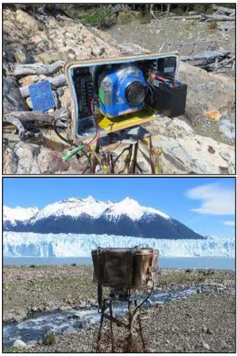
To support the field image acquisition, an integrated data acquisition system was built around the CANON EOS Mark II DSLR camera; pixel size: 7.2 µ, objective focal length: 50 mm, and FOV: 46°. The camera was calibrated several times, initially by the United States Geological Survey (USGS), and prior to field deployment. One of the recent camera calibration parameters obtained by using Photomodeler are listed in Table 1. The system is powered by two 12V/7Ah lead acid batteries, charged by two 38W solar panels. The camera with the supporting electronic systems is protected by a waterproof enclosure, with a viewing port and a visor to reduce reflections. An inspection port in the rear of the enclosure provides visual access to monitor status.
Focal Length 50.425 ± 0.014 mm Xp - principal point x 17.048 ± 0.011 mm Yp - principal point y 11.655 ± 0.012 mm
K1 - radial distortion 1 5.953e-005 ±8.8e-007 K2 - radial distortion 2 -2.007e-008 ± 6.6e-009 K3 - radial distortion 3 0.000e+000
Table 1. Camera calibration coefficients
The image acquisition system was installed on a rigid metal structure, fixed to outcrops of the shoreline of Lake Brazo Rico. The location, chosen in accordance with National Park requirements, provides a good side view of PM, see Fig. 2. The image acquisition started on April, 17 2012, and two pictures
per day were captured at 10 am and 8 pm local time for 368 days. In this study, five months of data, from 1st of October 2012 until 12th of February 2013 was used.
3.2 Ground support data
GPS determined Ground Control Points (GCPs) on a variety of topographic features were established in the field, including the camera projection center. Characteristic rocky outcrops were primarily preferred as they are assumed to be static in relation to the glacier. Double-frequency Trimble 5700 receiver measurements were referenced to the SGM (Station Glaciar Moreno) and SGU (Station Glaciar Upsala) CORS stations that are located at Brazo Rico lake and Upsala glacier. The computations were based on DGPS static positioning method. The results were converted to the POSGAR98 (Posicionamiento Geodésico Argentino) coordinate system (Lauria, 2009). The data was processing on Bernese software version 5.0 (Dach et al., 2007), using fixed solutions at the 95% confidence level. The RMSEs (root-mean-square error) for the GCPs were: RMS-N= 0.001m, RMS-E= 0.0008m, and RMS-U= 0.0025m; note that these numbers may be optimistic but that high level of accuracy is actually not required.
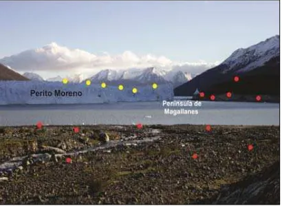
Six points on the glacier surface and three static points (inaccessible for measurement by GPS) were also captured, using the forward intersection method from two bases correctly georeferenced by GPS. The points taken into account were pinnacles of different heights, and the objective was to obtain the altitude of the glacier. The GCPs surveyed by total station had an RMS error of ± 30m; this is due to extreme base range ratio. Figure 3 shows the distribution of GCPs and checkpoints.
Figure 3. GCPs (red color) and check points (yellow color) distributed along the image.
3.3 Image correction
The overall processing workflow is shown in Fig. 4. In the first stage, the spatial resolution was calculated assuming a horizontal plane. With a 50mm focal lens and a pixel size of 7.2 microns, the size of the pixels for distances of 1,000, 1,500 and 2,000m was calculated to represent 0.14, 0.22 and 0.29m GSD, respectively. Although the internal geometries of the optical system are known and stable, lens distortions have an increasingly negative impact on accuracy as the target distance increases. The greatest geometrical distortions are radial, with lesser decentering components. The maximum radial distortion calculated near image corners is about 0.47m at the maximum distance of 2,000m. This error is largely mitigated by the fact that the area of interest is confined to the principal point in the right quadrant, resulting in a negligible error in this application.
Besides the optical errors, a second source of image correlation errors in our application is related to the physical displacement
of the camera system due to lack of perfect platform stability. Although the camera platform is a substantial structure, it is subject to short term disturbances in the form of wind buffeting and longer term changes, such as temperature effects on the support structure. These produce direct displacements of the sensor, making image correlation difficult. The image quality will also vary with precipitation, amount of sunshine and available daylight, all variables impacting the correlation accuracy. The GCPs provide a valuable asset in obtaining precise georeferencing to substantially improve data quality, and give quantitative data to assess the image data.
Figure 4. Workflow of the present study.
Images captured by the camera can be characterized by a number of factors. Assuming that an overall calibration is known for an individual instrument, the main factors are the position of the camera in the landscape (the principal point) and its orientation. If at least three GCPs are identified in the image, then the camera position and orientation can be determined, and a single camera can be used to collect quantitative image data. The 12 GCPs distributed across the image (Figure 3), clearly, increased the redundancy and provided for a robust image orientation solution. These points were projected onto the Argentine GK2 local mapping frame, and the first image frame was used as the reference. To assess and correct the effects of camera movement, least squares matching and 2D affine transformation model are used. Tie points were measured to allow stronger correlation between the image sequences, giving an RMS error of 1.2 pixels.
The difference in height between the target point and the camera center creates a scale error (Ahn & Box, 2010), which is also dependent upon the linear distance of the target from the camera. A number of checkpoints on the glacier surface were used to calculate the effect of relative height in terms of pixels in the image. Using an intersection method, the distance between the camera and a given object can be determined. This gives a measure of the relative heights allowing an estimation of the uncertainty of the scale factor assigned across the image. This uncertainty, at a maximum range of 1,800m in the area of the ice-dam collapse is in the order of around 5%. This results in a potential error of 50cm in a water level height of 10m. Known objects, for example a boat of known dimensions, also contributed toward quantifying scale factors. As the image capture reduces a 3D object space to a two dimensional image, relative movements will be greatly affected by the direction of travel relative to the camera. The movement in the study was at 45° with respect to the camera axis, resulting in a much greater uncertainty than the scale error.
3.4 Terrestrial validation
image effects, greyscale (monochrome) images were used, with three separate rock outcrops being digitized. The data captured was averaged, which significantly reduced the measurement error, and also temporally filtered to reduce errors from affects form waves and weather.
The results were correlated to daily direct measurements of Lago Rico by the Argentine Secretariat of Water Resources. The calculation of the Pearson’s r statistic (McKillup and Darby Dyar, 2010) demonstrated the strength of a linear relationship between the two variables, validating the accuracy of the method.
4. RESULTS
4.1 Testing TL technique
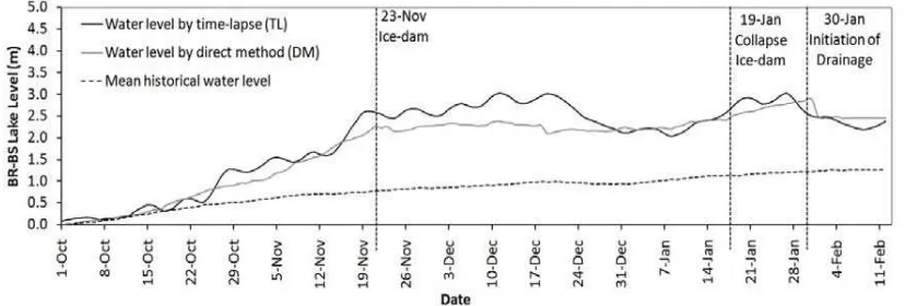
Over the 135 days of the study, the relative difference of water level in Lago Brazo Rico was 2.94 ±0.07m. Measurement from the time lapse equipment (TL) is shown by the black line, while the direct measurement (DM) values are indicated by the grey line. Direct measurement in the 1996-2001 and 2009-2011 periods, when no ice dam was present, is shown by the dashed black line. The effect of water retention by the ice dam is evidenced by the difference in levels. The data captured is shown in Figure 5.
Figure 4 shows TL data correlated to DM by Pearson coefficient. A score, Z, is assigned as equal to Z= µ and Xia set of data; µ is mean value and is the standard deviation. The Z scores increase similarly along a straight line. From this can be seen that the TL data matches the direct data well, with a value of r = 0.96, a mean of -0.009 and standard deviation of 1.004.
Figure 4. Distribution of TL and DM variables transformation (Z)
Figure 5. Water level trend of data taking by time lapse, direct method and mean water level without influence of ice-dam.
4.2 Glaciological results
The ice-dam tunnel started on 23th November, 2012, and the lake continued filling up to the date of rupture on 19 January, 2013. Even following the rupture, the level increased to a maximum on the 29 January. The following day, the lake had dropped by half a meter, showing loss from the rupture. The lake drained completely in February.
Ice-dammed lakes often exhibit temporary changes in behavior drainage as shown in Figure 5, generally in response to fluctuations of glaciers (Tweed & Russel, 1999). Once a critical threshold is reached (Paterson, 1994), the discharge mechanism will vary dependent on the topography of the lake basin, and the characteristics of the ice dam. This implies that a given drainage initiation mechanism may be specific to individual locations (Tweed & Russel, 1999).
The ice tunnel was studied from the 29 November until its final collapse on the 19 January. The width and height were
measured and the data presented in Figure 6. The tunnel form is roughly an ellipse. Initially, the tunnel produced a minimum height value of 5.2m and width of 21.5m. Over the tunnel’s life, the height increased to a maximum value of 22.3m; just three days prior to collapse. The tunnel width progressively increased to a maximum value of 54.5m, related to lateral undermining. This was followed by rapid changes in the tunnel morphology until the final collapse event.
point that structural failure results, also releasing ice into the water.
Figure 6. Height and width evolution of the tunnel.
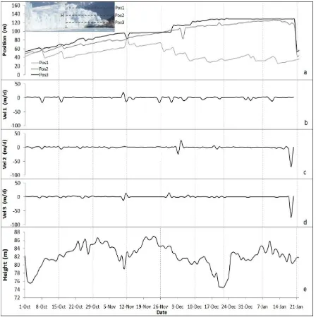
In this study the height of the glacier front of the PM was recorded close to the tunnel zone. 113 images were captured in a daily sequence showing positions 1, 2 and 3 in the frontal area, and the heights recorded. The mean height of the glacier front was determined to be 75m. The data is presented in Figure 7.
Figure 7a shows the effects that occur when the glacier heads toward, and abuts the Peninsula de Magallanes. The top of the glacier moves faster than the lower sections, causing shear zones to develop along an arcuate surface. The mean advanced of position 1 was 47.15m ±2.35m during the studied period. The mean velocity was of -0.10m/d ±0.005m. It has the greatest calving effect that can be shown in each fracture almost equidistantly along the path. The values show sudden peaks associated by calving and an increment in the trend occur when the ice-dam collapse. Positions 2 and 3 have similar trends, described as a front advance; the mean velocities are 0.58m/d ±0.03m and 0.67m/d ±0.003m, respectively. These results are according to Ciappa et al. (2010) where velocity maps of the front of PM was obtained by cross correlation SAR imagery in November of 2009. Figure 7e shows the height variation. The evolution shows drastic changes experienced due to calving. The peaks in a higher position had a height of 86.99m ±4.35m, reached due retreat experience; in some cases, it was up to 10m.
5. CONCLUSIONS
In this study, the feasibility of time lapse terrestrial photogrammetry for glaciological applications was demonstrated. The cost effectiveness of the technique coupled with the simple data acquisition and subsequent processing provided a valuable spatial/temporal resolution to monitor glaciers. The technique was correlated and validated by manually digitizing the level height against daily direct measurement of Lago Rico, obtaining a Pearson coefficient of 0.96, indicating a good match between the two variables. The results have shown acceptable quality and accuracy estimation of elevation and planimetric changes of the glacier. The analysis of daily velocities suggests that calving events are mainly determined by the movements in the front area, where the glacier moves toward to the front; this effect may produce negative velocities of -0.10m/d. The photogrammetric processing, including scale factor estimation errors, could be improved by using daily data from another camera view; stereo or even multi-ray image processing. Also, the data collected can be further verified from other techniques, such as satellite photogrammetry, LiDAR or SAR to give a high level of confidence.
ACKNOWLEDGEMENTS
The authors would like to thank Pedro Skvarca for his advice, Simon Key for his help in the English version, and Adalberto Ferlito for field assistance. Robert Smalley Jr. (Univ. of Memphis, USA) provided the PS GNSS data. Parque Nacional Los Glaciares provided support in the area. Fieldwork was funded by grant PICT 2921-2012, Agencia Nacional de Ciencia y Tecnología Argentina (ANCyT).
REFERENCES
Ahn, Y. & Box J. E., 2010. Instruments and Methods. Glacier velocities from time-lapse photos: technique development and first results from the Extreme Ice Survey Greenland. Journal of Glaciology, 56: 198.
Aniya, M. and Skvarca, P., 1992. Characteristics and variations of Upsala and Moreno glaciers, southern Patagonia,” Bulletin of Glacier Research, 10: 39-53.
Aniya, M., Sato, H., Naruse, R,. Skvarca, P., and Casassa, G., 1996. Remote sensing application to inventorying glaciers in a large, remote area-Southern Patagonia Icefield. Photogrammetric Engineering and Remote Sensing, 62: 1361-1369.
Ciappa, A., Pietranera, L., and Battazza, F., 2010. Perito Moreno Glacier (Argentina) flow estimation by COSMO SkyMed sequence of high-resolution SAR-X imagery, Remote Sens. Environ., 114(9): 2088–2096.
Dach, R., Hugentobler U., Fridez P., and Meindl M., 2007. BERNESE GPS Software Version 5.0. Astronomical Institute, University of Bern, Berna.
Danielson, B. and Sharp, M., 2013. Development and application of a time-lapse photograph analysis method to investigate the link between tidewater glacier flow variations and supraglacial lake drainage events. Journal of Glaciology 59: 287-302.
Hanson, B. and Hooke, R., 2000: Glacier calving: a numerical model of forces in the calving-speed/water-depth relation. Journal of Glaciology, 46(153): 188-196.
Harrison, W.D., K.A. Echelmeyer, D.M. Cosgrove and C.F. Raymond. 1992. The determination of glacier speed by time-lapse photography under unfavourable conditions. Journal of Glaciology, 38(129): 257–265.
Lauria, E.A., 2009: República Argentina–Adopción del Nuevo Marco de Referencia Geodésico Nacional POSGAR 07– RAMSAC. Novena Conferencia Cartográfica Regional de las Naciones Unidas para América, United Nations E/CONF.99/CRP.9, New York, 10–14 August.
McKillup and Darby Dyar, 2010. Geostatistics Explained An Introductory Guide for Earth Scientists. pp389.
Maas H.G., Casassa G., Schneider D, Schwalbe E, and Wendt A., 2010. Photogrammetric determination of spatio-temporal velocity fields at Glaciar San Rafael in the Northern Patagonian Icefield. The Cryosphere Discussions. 4, 2415–2432.
Paterson, W., 1994. The Physics of Glaciers. 2nd Edition. Pergamon Press. Oxford, New Cork, Seoul y Tokio, pp 385.
Rivera, A., Corripio, J., Bravo, C., and Cisternas, S., 2012. Glaciar Jorge Montt dynamics derived from photos obtained by fixed cameras and satellite image feature tracking, Annals of Glaciology, 53: 60A152.
Shan, J. & Toth, C., 2008. Topographic Laser Ranging and Scaning: Principles and Processing. CRC Press, Taylor and Francis.
Svanem, M., 2010. Terrestrial Photogrammetry for velocity measurements of Kroneebreen calving front. Master Thesis, Norwegian University of Life Sciences.
Tweed, F. & Russel, A., 1999. Controls on the formation and sudden drainage of glaciar-impounded lakes: implications for jökulhlaup characteristics. Progress in Physical Geography, 23 (1): 79-110.