Brine transport in porous media: self-similar
solutions
C.J. van Duijn
a, L.A. Peletier
b& R.J. Schotting
c ,*
aP.O. Box 94079, 1090 GB Amsterdam, The Netherlands b
Mathematical Institute, Leiden University, P.O. Box 9512, 2300 RA Leiden, The Netherlands c
Department of Watermanagement, Environmental and Sanitary Engineering, Delft University of Technology, P.O. Box 5048, 2600 GA Delft, The Netherlands
(Received 28 October 1996; revised 10 March 1998; accepted 20 March 1998)
In this paper we analyze a model for brine transport in porous media, which includes a mass balance for the fluid, a mass balance for salt, Darcy’s law and an equation of state, which relates the fluid density to the salt mass fraction. This model incorporates the effect of local volume changes due to variations in the salt concentration. Density variations affect the compressibility of the fluid, which in turn cause additional fluid flow. Two specific situations are investigated that lead to self-similarity. We study the relative importance of the compressibility effect in terms of the relative density difference. Semi-analytical solutions are obtained as well as asymptotic expressions in terms of the relative density difference. It is found that the volume changes have a small but noticeable effect on the mass transport only when the salt concentration gradients are large. Some results on the simultaneous transport of brine and dissolved (radioactive) tracers are presented.q1998 Elsevier Science Limited. All rights reserved
Keywords: brine transport, compressibility, similarity transformations, porous media, 35K55, 76S05.
1 INTRODUCTION
Recently Hassanizadeh and Leijnse1–3revisited the theory of brine transport in porous media, designed numerical codes and did experiments in the laboratory. They raised the question whether (semi-) analytical solutions of the governing equa-tions could be obtained under certain boundary and initial conditions. This question initiated our mathematical study and the results are published in the mathematics literature4. Because the subject of brine transport is still of current interest in the hydrological literature and the availability of analytical work in this field is poor, we decided to make the mathema-tical results more accessible for non-mathematicians and wrote this paper. The material has been extended with new results and the emphasis is now on the construction of semi-explicit self similar solutions.
Brine is water containing a high concentration of salt. In an almost saturated brine the mass fraction (q), which is
defined as the mass of the salt per unit mass of brine, can reach 0.26. This corresponds to a brine density of approxi-mately 1200 kg m¹3. For sea waterq¼0.04 corresponding to a fluid density of 1025 kg m¹3. Mass fraction and density are related by an equation of state, which has been empiri-cally determined. Brines are found in surface waters, such as the Dead Sea, and groundwater near salt domes5. These are geological structures in the subsurface consisting of massive bodies of salt, a kilometer or more in diameter, embedded in horizontal or inclined strata. Salt domes are potential places for storage of nuclear waste6, and it is of practical impor-tance to know the flow of the groundwater around them.
Any model for fluid flow and salt transport in a porous medium must contain the mass balance equations for the fluid and the salt, and Darcy’s law. The specific model we propose to study uses the fluid mass balance equation1
f]r
]tþdiv(rq)¼0 (1)
where f denotes the porosity of the medium, r the fluid density and q the specific discharge vector. Introducing the
Printed in Great Britain. All rights reserved 0309-1708/98/$ - see front matter
PII: S 0 3 0 9 - 1 7 0 8 ( 9 8 ) 0 0 0 0 8 - 6
285
material derivative
D Dt¼
] ]tþ
q
f·grad (2)
in the balance equation yields
f r
Dr
Dtþdivq¼0 (3)
This expression shows that density variations may affect the compressibility of the fluid, which in turn can affect the fluid motion. To make this effect explicit is one of the goals of this study.
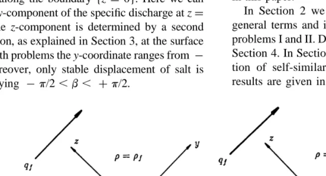
In this paper we intend to employ mainly analytical techniques. Therefore, we are forced to restrict ourselves in the choice of flow problems. Inspired by earlier work of de Josseling de Jong and van Duijn7we shall analyze two simplified cases denoted by Problem I and Problem II. Problem I describes the mixing of fresh water and brine, originally separated and flowing parallel, due to transversal dispersion. Problem II relates to the flow of groundwater along the surface of a salt dome. A sketch of the correspond-ing initial and boundary conditions is given in Fig. 1. In Problem I the flow domain is unbounded above and below. Initially, say at t¼0, the region above the plane {z¼0} is filled with fresh water and the brine fills the region below it. In this case one has to specify the specific discharge either as
z→ þ`or as z→ ¹`. Here we shall adopt the former, and fix q→(qƒ,0) as z→ þ`, where qƒis a given constant. In Problem II the flow domain consists of the upper half space {z . 0} and is bounded below by an impermeable salt rock.
Again at t¼0, fresh water occupies the region {z.0} while the salt from the rock ensures thatr¼rs(mass density of saturated brine) along the boundary {z¼0}. Here we can only specify the y-component of the specific discharge at z¼ þ`, because the z-component is determined by a second boundary condition, as explained in Section 3, at the surface of the rock. In both problems the y-coordinate ranges from ¹
` to þ `. Moreover, only stable displacement of salt is considered, implying ¹p/2,b, þp/2.
These problems are chosen because they admit to look for similarity solutions. This means that the underlying partial differential equations can be reduced to ordinary differential equations by introducing an appropriate similarity variable (e.g. z=pt in Fig. 1). This makes the analysis tractable,
yielding semi-explicit results. The mathematical justifica-tion of the results is given elsewhere4. As a consequence of the analysis we can quantify the effect of the additional brine transport due to the fluid compressibility for Problems I and II, where in particular the latter is relevant to under-stand the flow near salt domes.
Among recent papers focusing on brine transport we mention Oldenburg and Pruess8; Carey et al.9, Herbert et al.10, Hassanizadeh and Leijnse3. Numerical codes1,2 are developed to simulate flow of groundwater containing high salt concentrations. There are only few high-concen-tration brine transport experiments available for testing the validity of numerical codes. Our (semi) analytical results can be used to verify the accuracy of numerical codes11,2. Herbert et al.10stresses the importance of analytical work on this subject.
In the literature, the validity of Darcy’s law and Fickian dispersion equations for high concentration differences has been questioned. For example, Hassanizadeh and Leijnse3 reported on column tests of brine displacing fresh water in a porous medium. They showed that the dispersivity of brine decreases when the relative density difference between brine and fresh water increases and resolved this problem by introducing a non-linear form of Fick’s law. Carey et al.9 suggest a density dependent diffusivity–dispersivity. Although these results are interesting we shall confine our-selves to the classical formulation of Fick’s and Darcy’s law in this paper.
In Section 2 we formulate the mathematical model in general terms and in Section 3 we define the two specific problems I and II. Dimensionless variables are introduced in Section 4. In Section 5 we discuss properties and construc-tion of self-similar soluconstruc-tions. Numerical procedures and results are given in Section 6 while asymptotic results for
small relative density difference, yielding approximately div(q) ¼0, can be found in Section 7. The simultaneous transport of brine and dissolved radionuclides is the subject of Section 7. In Section 8 we discuss the results and Section 9 contains the conclusions.
2 THE MATHEMATICAL MODEL
Since this paper focuses on analytical aspects of subsurface brine transport, we shall impose simplifying restrictions on the properties of the porous medium and flow. With respect to the porous medium we assume that it is homogeneous and isotropic, characterized by a constant porosityfand intrin-sic permeabilityk. With respect to the flow we shall con-sider the two specific cases which are introduced in Section 1 and about the fluid, with densityrand salt mass fractionq, we assume that the dynamic viscositymdoes not depend on qand is constant.
Assuming a Fickian type of dispersion–diffusion term in the salt mass flux and restricting ourselves to the conven-tional form of the momentum balance equation, we obtain the following equations for transport of brine1:
Mass balance of the fluid
f]r
]tþdiv(rq)¼0; (4)
Mass balance of the salt
f]rq
]t þdiv(rqq)¹Drgradq¼0; (5)
Darcy’s law m
kqþgradp¹rg¼0; (6) Equation of state
r¼rƒegq (7)
Here q¼(qy,qz) denotes the specific discharge, p the fluid pressure and g¼(gy,gz) the acceleration of gravity. In the equation of state, where we disregard the effect of pressure variations on the fluid density,rƒis the density of the fresh water andgis a constant (g¼0.6923<ln 2) obtained by
curve fitting using a table from Weast12. Following Bear13, the hydrodynamic dispersion tensor D¼(Dij) is given by the expression
Dij¼{aTlqlþfDmol}dijþ(aL¹aT)qiqj=lql (8)
whereaLandaTare positive constants withaL.aT. They are called the longitudinal and transversal dispersion length, and describe the spreading of solutes due to mechanical dispersion caused by randomness of the struc-ture of the porous material and heterogeneities. Further
Dmol denotes the effective molecular diffusivity, which incorporates the effect of tortuosity. Finally, dij denotes the Kronecker d and l·l the Eucidian norm in R2. For
mathematical reasons we use in most of this paper (except in Section 9) the approximation
Dij¼fDdij (9)
where D is a positive constant.
3 THE FLOW PROBLEMS
The object of any study of brine transport is to determine the specific discharge and density (or mass fraction of salt) of the fluid as a function of position and time. We will investigate here two specific problems. In Problem I, see Fig. 1(a), we consider an unbounded flow domain above and below the z¼0 plane. Initially, at time t¼0 say, the region above this plane is filled with fresh water (density rƒ) and the region below it with brine (densityrs). Sincers . rƒand assuming ¹p/2,b, þp/2, this leads to a stable salt distribution for all t$ 0. As a boundary con-dition we impose that at large distance above the z ¼0 plane, the flow is known (and given) and points into the y-direction:
q→qƒey as z→ þ`, for all t$0 (10)
where qƒis a given constant and eythe unit vector in the positive y-direction.
Studies of brine distributions in aquifers have shown that the transition zone between brine and fresh water is rela-tively narrow, in particular when the fluids are stagnant. If this situation is perturbed by draining fresh water we end up with a situation that can be represented schematically by Problem I.
In Problem II the flow domain occupies the half space {z . 0}, see Fig. 1(b). In formulating this problem we have
assumed the initial situation where, due to regional effects, fresh groundwater flows along the top boundary of a salt dome. As a result salt will dissolve from it. The physico-chemical processes that take place at a salt rock boundary are complex and difficult to model. For instance, the dissolution of salt creates a cap (residue) rock layer along the top of the salt dome. Geological studies, e.g. Bornemann et al.14, estimate the growth of this layer to be 0.04 mm year¹1. Following Hassanizadeh and Leijnse1 we disregard this movement and assume that the mass fraction remains at all times at the maximal salt mass fraction of the saturated brine along the fixed boundary, i.e.
q¼qs at z¼0, for all t$0 (11)
Further, the flux of salt entering the flow domain induces a movement of water. This leads to the additional boundary condition, see again Hassanizadeh and Leijnse1,
(qþ D
(1¹qs)
gradq)·n¼0 at z¼0, for all t$0 (12)
where n denotes the outward normal at the boundary {z¼
everywhere in the flow region. At large distance above the {z¼0} plane we now impose only the y-component of the flow, since the z-component will be determined by the pro-blem. Thus we set
qy→qƒ as z→þ`, for all t$0 (13)
In both problems the y-coordinate ranges from ¹`to þ `. Therefore, we may look for a density and specific
dis-charge depending only on the z-coordinate and time, i.e.
r¼r(z,t)and q¼q(z,t) (14)
This assumption implies irrotational flow in both problems. We do not consider perturbations of the initial condition on r. Following de Josseling de Jong and van Duijn7we use eqn (14) and Darcy’s law (eqn (6)) to obtain a linear alge-braic relation between the fluid density and the y-compo-nent of the specific discharge. This relation can be found by first taking the curl of eqn (6):
]
and by substituting eqn (14) into this expression. The result is
wherebis the inclination of the z¼0 plane. To determine the constant in eqn (16) we use the behavior of qyandrat z
¼ þ`:
qy(`,t)¼qƒ andr(`,t)¼qƒfor all t.0 (17)
This yields the relation
qy¼qƒ¹
k
m(r¹rƒ)gsinb (18) Thus in order to determine the pair (r,q) from the differ-ential equations with initial and boundary conditions, there remains by virtue of eqn (18), only to determiner and qz. Using eqn (18), the equations for these quantities reduce to
f]r
Combining these equations yields
fr]q
and with the equation of state (eqn (7)) we obtain
f]r
We use the couplied system eqns (19) and (22) in our analysis. To determinerand qzfrom this system we need
to impose the initial and boundary conditions. In Problem I we look for a solution in the domain {(z,t):¹` ,z, þ `, t .0} subject to the initial condition
r(z,0)¼ rf
for z.0
rs for z,0
(
(23)
and boundary condition eqn (10) for the flow
qz(þ`,t)¼0 for all t$0 (24)
We note that a condition on the flow such as eqn (24) is natural for the problem. Combining eqns (19) and (22) gives the ordinary differential equation
r]qz ]z þD
]2r
]z2¼0 (25)
Thus knowingr, a single condition on qz[e.g. Eqn (24)] is needed to determine the solution. The specific choice is arbitrary. In fact one could construct a solution corresponding to any given qz( þ `,t). We also observe at this point that eqn (25), when writing it in the form
div q¼]qz
]z¼ ¹
1
rdiv(Dgradr) (26)
clearly demonstrates the coupling between brine transport by diffusion–dispersion, creating a non-zero divergence in the flow field, and hence enhanced fluid flow. Density gradients imply fluid movement and vice versa.
Problem II is solved in the domain {(z,t): z .0, t .0} where we impose initially
r(z,0)¼rf for z.0 (27)
and along the boundary, see eqns (11) and (12)
r(0,t)¼rsm:¼rfegqs (28)
4 DIMENSIONLESS VARIABLES
Before discussing eqns (19) and (22) we introduce the dimensionless variables
terms of these new variables the equations become (drop-ping the asterisks notation)
]r
The rescaled initial and boundary conditions in Problem I are
In Problem II the scaling eqns (30) and (31) lead to r(z,0)¼0 for z.0 (36)
Note that the relative density differences lies in the interval
0, « ,egqs¹1
<2qs¹1<0:2 (40)
forqs¼0.26
5 SELF-SIMILAR SOLUTIONS
Due to the non-linear coupling between eqns (32) and (33) it is not possible to find explicit, closed-form solutions of Problems I and II. Nevertheless, their special structure enables us to obtain much information concerning the
qualitative behavior of the solutions and to obtain accurate approximations.
The key idea is to look for self-similar solutions, which reduce eqns (32) and (33) to a set of coupled ordinary differ-ential equations with boundary conditions originating from eqns (34)–(38). The transformed problems were studied in detail by van Duijn et al.4. They considered fundamental questions related to existence and uniqueness of solutions, as well as their qualitative behavior. With respect to the latter, they showed certain monotonicity properties of solu-tions and their asymptotic behavior forlzl→`and for«↓0. Some of these results will be discussed here and in Section 7. The similarity transformations for Problems I and II are given by
This results in the set of differential equations
(uv)9þ1
where the primes denote differentiation with respect to h. The independent variable h ranges from ¹`to þ`in Problem I and from 0 to þ`in Problem II.
The following boundary conditions for u(h) and v(h) in Problem I result from eqns (34) and (35) and are found to be
u(¹`)¼1 and u(þ`)¼0 (45)
and
v(þ`)¼0 (46)
For Problem II we find from eqns (36)–(38)
u(0)¼1 and u(þ`)¼0 (47)
and
v(0)¼ ¹K(«)«u9(0) (48)
Eqns (43) and (44) can be combined into:
u0þ 1
Let us first discuss Problem I. We start with the important observation that solutions (u,v) of equations eqns (49) and (50) on R are invariant under linear shifts. By this we mean the following. For any given a[ R, let
¯h¼h¹a, u¯(¯h)¼u(h)andv¯(¯h)¼v(h)¹1
2a (51) Then if [u(h),v(h)] solves eqns (49) and (50) for ¹` ,h
(49). This means that if [u(h),v(h)] is a solution for which
v(6 `) exists, then by shiftinghover a suitable distance
a, we can reach any limiting value of v(h), either ath ¼ ¹`or at h ¼ þ`. If we choose a ¼2v(þ`) in eqn (51) we can ensure that eqn (46) is satisfied. This invariance property will be used in both the mathematical and numerical procedures for solving Problem I.
Before discussing the construction of solutions, we recall some a priori properties which give an idea about the qualitative behavior of the solution. We proved in Van Duijn et al.4that
1. u9(h), 0 for all ¹` , h, þ`;
2. there existsh0.0 such that u0(h),0 forh,h0and
u0(h). 0 forh. h0
3. v(h0)¼12h0and v9(h).0 forh,h0and v9(h),0 for
h .h0
4. u9(h)→0 iflhl→`
The first assertion implies that the brine concentration increases strictly with depth and is concave below the plane z¼h0
t
p
and convex above it. Also the z-component of the specific discharge has a maximum at
z¼h0
t
p
of magnitude qz(h0sqtt,t)¼12h0=
t
p
. The number h0 plays a prominent role in simultaneous transport of brine and radionuclides, which will be explained in Sec-tion 8.
Next we turn to the solution procedure. As a first obser-vation we note that eqns (49)–(51) can be combined into a single equation withh missing. This equation, having the form
1 2þ
u0
u9
9¼ ¹ u0 uþ1
«
with ¹` ,h, þ` (52)
needs three conditions to be solved uniquely. Two conditions are given by eqn (45). As a third condition we take, for instance,
u(0)¼1
2 (53)
We outline below how to obtain a unique solution satisfying eqns (52), (45) and (53) and how to obtain from that solution a corresponding v ¼ v(h) so that the pair (u,v) satisfies eqns (43) and (44). This function v will not satisfy eqn (46). To achieve that condition one applies the linear shift (eqn (51)) with a¼2v(`).
Eqn (52) is of third order, non-linear and defined on an unbounded domain. To tackle it directly is, therefore, not straightforward. As so often in mathematics, we solve problems by combining and applying what we already know. Also in this case, we will transform eqn (52) into a second order equation on a finite domain, yielding a boundary value problem which is well known in the mathematical literature. This transformation is achieved by taking u as the independent variable, which is allowed
by the monotonicity of u, and by taking u9 as the new independent variable. Thus setting
h¼h(u)and y(u)¼ ¹u9(h(u)) (54)
we obtain
y{(1þ«u)y9}9¼ ¹1
2(1þ«u), 0,n,1 (55)
In view of property (4) we obtain for y the boundary con-ditions
y(0)¼0 and y(1)¼0 (56)
By setting further
s¼log(1þ«u)
log(1þ«) and z(s)¼ «
log(1þ«)y(u) (57)
we obtain the problem
(I9) ¹zz
0¼1 2e
2slog(1þ«),
z.0 for 0,s,1
z(0)¼z(1)¼0 (
(58)
which is well known and arises in the study of self-similar solutions of non-linear diffusion equations, see for instance Esteban et al.15, Van Duijn and Peletier16, Van Duijn and Floris17and Van Duijn et al.18. In the context of nonlinear diffusion one calls eqn (58) the flux equation, because it specifies the flux in terms of the concentration. One sees immediately (since z. 0) that
z0(s),0 for 0,s,1 (59)
Less straightforward are the proofs of the properties
lim
s↓0 z
9(s)¼ þ`and lim
s↑1 z
9(s)¼ ¹` (60)
which can be found in Van Duijn and Floris17. Knowing that a solution z ¼ z(s) of Problem I9 exists and is unique, and knowing much about its qualitative behavior, one finds y¼y(u) from eqn (57). Finally, the solution u¼ u(h) satisfying eqns (52), (45) and (53) is implicitly defined by
h(u)¼ Z12
u
1
y(s)ds (61)
which results from integrating eqn (54). The corresponding
v¼v(h) is given by
v(h)¼1
2h¹y9(u(h))for ¹` ,h, þ` (62)
which follows from eqns (49) and (54).
picture of the solution. The solution procedure proceeds along the same lines. It leads to the transformed problem
(II9) ¹zz0¼
where L is a constant given by
L¼K(«)(1þ«)log(1þ«)¼ log(1þ«)
g¹log(1þ«) (64) The boundary condition at s¼1 is a direct consequence of eqn (48). To return to u¼u(h), we first use again eqn (57)
The corresponding v¼v(h) is obtained from eqn (62).
6 NUMERICAL PROCEDURES AND RESULTS
The mathematical analysis has provided us with qualitative information about the structure of the solutions of Problem I and II. This information can be used to develop procedures to obtain accurate numerical solutions.
Starting point for both problems is the third order eqn (52). We write this equation as a system of first order equa-tions by setting
p¼u, q¼u9and r¼v (66)
Substitution in eqn (52) yields
(S)
To solve this system we impose three conditions ath¼0:
p(0)¼u(0)¼p0, q(0)¼u9(0)¼q0, r(0)¼v(0)¼r0
(68)
where p0 ¼1/2 (Problem I) or p0¼ 1 (Problem II), and where q0 and r0 are a priori unknown. They have to be determined from the boundary conditions eqn (45) (Pro-blem I) or from eqns (47) and (48) (Pro(Pro-blem II).
Concerning Problem I, one approach is to apply a shoot-ing procedure in the regions {h,0} and {h.0}. Taking for (S) the initial values p0¼1/2 and q0, r0arbitrary, one solves the equations for {h,0} and {h.0}. The idea is to choose p0and q0such that
p(¹`)¼u(¹`)¼1 and p(þ`)¼u(þ`)¼0 (69)
However, this procedure is not at all trivial because there
are two degrees of freedom in the problem. Moreover, it would be time consuming to compute accurate values for q0 and r0 by trial and error such that the correct limiting behavior for u at h¼ þ/ ¹`is achieved.
An alternative approach is to determine q0and r0directly from Problem (I9) by noting that
p0¼ ¹y
and, using eqn (48),
r0¼ ¹y9(1
We find approximate values of the shooting parameters q0 and r0by solving (I9) numerically. We omit the details of the computations. Next equations (S) are solved using a fourth order Runge–Kutta method in the regions {h ,0} and {h. 0}, subject to p0, q0and r0. This gives the solu-tion [u(h), v(h)] of eqns (49) and (50) which satisfies
u(0)¼1=2. It also provides us with the value of v(þ`)¼
r(þ`) which we need to obtain the correct shift a ¼ 2v(þ`) to satisfy boundary condition eqn (46).
In all cases considered, i.e. for all relevant values of«, we verified the boundary conditions u(þ`)¼0 and u(¹`)¼
1. Up to a small error term ( < 6 10¹6) these values are reproduced by the numerical approximations. This serves as an independent check for the accuracy of the numerical procedure for Problem (I9).
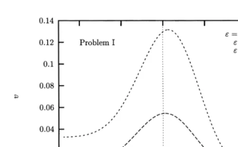
Figs 2 and 3 give the results of the numerical approxima-tions of the similarity soluapproxima-tions u(h) and v(h) for different values of the relative density difference«.
The value«¼0.025 corresponds to sea water. This curve is not distinguishable from the curve for«¼0 on the scale of Fig. 2. The limit«→0 is the so-called Boussinesq approxi-mation of Boussinesq limit, see Section 7. The value«¼0.2 corresponds with an almost saturated brine, while « ¼ 0.5 (although physically not possible) is chosen here to empha-size the effect. Observe that the numerical solutions satisfy the qualitative behavior discussed in Section 5.
Concerning Problem II we solve system (S) for h . 0 subject to the initial conditions
p(0)¼u(0)¼1 (72)
q(0)¼u0(0)¼q0,0
r(0)¼v(0)¼ ¹«K(«)q0
where the last condition is a consequence of eqn (48). This is a one-parameter shooting problem which is more straightforward and is solved without using Problem (II9). The object is to find an approximate value of q0such that the boundary condition u( þ `) is satisfied. This can be achieved by starting the shooting procedure with an initial estimate for q0 and check if the corresponding limiting behavior is satisfied at sufficiently large distance L from the origin. The problem is to determine an approximate value of q0such that the boundary condition u( þ`)¼0 is satisfied. This can be achieved by starting the shooting procedure with an estimated value of q0 and check if the corresponding limiting behavior is satisfied at a sufficiently large distance L from the origin. If u(L).d.0, wheredis an a priori specified small error term, the estimated value of
q0 is decreased by a fixed amount Dq0 and the shooting procedure is repeated. The step size Dq0 remains fixed until, say after the nth step, un(L),0. Now qn0 is increased by the bisection ofDq0, hence q(
nþ1) 0 ¼q
0
0¹Dq0(n¹(1=2)).
If unþ1(L).dor if unþ1(L),0 we bisect the last alteration
of q0 again and obtain, respectively: q
nþ2 0 ¼q
0 0¹
Dq0(n¹(1=4)) or q
nþ2 0 ¼q
0
0¹Dq0(n¹(3=4)). This
proce-dure is repeated until 0# u(L)# d. The number of steps depends on the quality of the initial guess of q0 and the initial step sizeDq0.
Fig. 4 shows the results of the iterative shooing procedure for the scale density u(h) for different«-values. The corre-sponding scaled specific discharge distributions v(h) are given in Fig. 5. Notice that v(0)Þ0. This is a consequence of boundary condition eqn (48) at the salt rock–brine inter-face. Because u is a decreasing function we have u9(0),0, hence v(0).0, for all« .0.
Figs 6 and 7 give the relative densityr(z,t)¼u(z=pt)and
the unscaled specific discharge qz(z,t)¼v(z=
t
p
)=ptat
dif-ferent time levels in the original variables. The other para-meter values used in these examples are adopted from Herbert et al.10and listed in Table 1.
Remark (boundary condition): If we impose, instead of eqn (48), the condition qz(0,t)¼0 for all t.0 to express the assumption that the salt rock boundary is impervious, then the analysis yields v(h),v(0)¼0 for allh.0. An expla-nation for this behavior is that qz¼0 at the boundary can only be maintained by a back flow coming from þ`. We conclude that this is a physically unrealistic situation and that the no flow boundary is incompatible with the model discussed in this paper.
Fig. 3. Numerical approximations of v(h) for Problem I.
Fig. 4. Numerical approximations of u(h) for Problem II.
Fig. 5. Numerical approximations of v(h) for Problem II.
Some results of a formal asymptotic analysis are given in the Appendix A of this paper. This analysis yields series expansions in terms of the relative density difference«for the similarity solutions u(h) and v(h). When these expan-sions are truncated we obtained approximation formulas, up to a certain (known) accuracy.
7 TRANSPORT OF RADIONUCLIDES
In this section we consider the simultaneous transport of a non-adsorbing radionuclide, occurring in tracer concentra-tions, in the vicinity of a salt dome. We assume that the flow geometry is given by Problem II, resulting in one-dimen-sional (z-direction) transport. The equation to be solved is
Rf]rqc
whereqcdenotes the mass fraction of a radionuclide,lthe decay constant, R the retardation factor for linear equili-brium adsorption, and Dc its effective diffusivity–disper-sivity. Note that qz¼qz(z,t) andr¼r(z,t) are solutions of Problem II. Further, note that in general DcÞ D, the dif-fusivity of the salt. We introduce the parameterv, defined as
v¼Dc=D (74)
and apply the scaling rules eqn (30) in eqn (73). This ensures identical time scales for brine and radionuclide transport. The radionuclide mass fraction is scaled accord-ing to
where q0 denotes a reference mass fraction, e.g. the
(radionuclide) mass fraction at the salt rock boundary. As a consequence of eqn (30) we find
lp¼ RfD
k mrfg
2l (76)
as the dimensionless decay constant. Combining eqns (73) and (19), and applying eqns (30), (74)–(76), we obtain (omitting the asterisks)
in which we eliminated the decay term in the usual way, i.e. by setting qc(z,t)¼q¯c(z,t)e¹lt. The boundary and initial eqns (77) and (78) have a self similar solution
¯
To solve this problem we first elimniate v using eqn (49) and next integrate the resulting equation. This leads to
f(h)¼1¹
where u is the solution of Problem II, for a given value of«. The corresponding, scaled radionuclide concentration is
¯
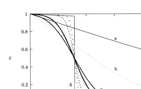
Fig. 8 shows the scaled concentrationc for different values¯ ofvand«¼0.2. The results in this figure indicate that, asv Fig. 7. Specific discharge at different times for«¼0.2 in Problem II.
Table 1.
Property Value Physical unit
→0, the concentration c has a discontinuity at¯ h ¼h0<
0.316 withc¯¼0 forh.h0. This is a direct consequence of the limiting behavior of (BVP) asv→0: i.e.
ƒ9(v¹h
2)¼0 for all h.0
ƒ(0)¼1, ƒ(`)¼0 8
<
:
(83)
which implies a piecewise constant solution
f(h)¼ 1 for 0
,h,h0 0 for h.h0 (
(84)
and thus
¯
c(h)¼
«u(h)þ1
«þ1 for 0,h,h0 0 for h.h0 8
<
:
(85)
As a consequence, a radionuclide front emerges which moves with speed v(h0=
t
p
), where v(h) ¼ max((v(h)) ¼
h0/2, see property (3) in Section 5. The position of the front in the (z,t)-plane is given by
s(t)¼2v(h0)
t
p
¼h0
t
p
, which is equivalent to the path of a tracer particle released at t ¼ 0 in z¼ 0, i.e. at the beginning of the brine transport process. Hence in the limit v→0, the movement of the tracer is caused by the com-pressibility effect only.
8 DISCUSSION
Self-similar solutions make the analysis tractable and (semi-) explicit results can be obtained. A crucial requirement for the applicability of similarity arguments is that both the governing equations and initial and/or boundary conditions be reducible to the similarity form. Hence, only in special cases one may expect to find similarity solutions. Due to the piecewise initial density distribution in Problem I and II we may consider the obtained similarity solutions as upper lim-its for the compressibility effect. Smooth initial data decrease the magnitude of the enhanced flow.
In analyzing Problems I and II we show explicitly the effect of enhanced groundwater flow due to compressibility of fluid caued by high salt concentration gradients. Charac-teristic for both problems is the occurrence of additional specific discharge in a direction perpendicular to the main groundwater direction. In both problems qzis not influenced by gravity. The only quantity that depends on gravity is the specific discharge in the y-direction, parallel to main flow
qƒ.
The flow geometry of both problems and the boundary– initial conditions are chosen such that semi-analytical solu-tions are obtained. These solusolu-tions allow us to study the relative importance of volume effects in terms of the rela-tive density difference. Although the flow of groundwater in the vicinity of a ‘real’ salt dome is more complex, the sim-plified problems studied in this paper gain insight in the non-linear coupling between fluid density and fluid flow due to volume effects.
The salt rock boudary condition, which relates the fluid mass flux to the diffusive–dispersive mass flux at the salt boundary, is physically more realistic than the often used no-flow condition qz(0,t) ¼ 0. The latter induces a back flow coming from z¼ þ`to maintain the no-flow condi-tion at z¼0, see the remark in Section 6.
In this paper we only consider constant (molecular) diffu-sion. In a more realistic description a velocity dependent dispersion matrix has to be introduced into eqn (5). Mole-cular diffusion underestimates the compressibility effects.
When transversal dispersion, due to the (regional) back ground flow qy, dominates the dispersion–diffusion in the z-direction we arrive at a different situation. Under the assumptionlqzl,lqyleqn (8) reduces to
D<fDmolþaTlqyl¼ (86)
fDmolþaTlqƒ¹
k
m(r¹rƒ)gsinbl (87) yielding D as a function of r. The analysis of this case is quite different from what we discussed here and will be published elsewhere18.
If qƒq
k
m(rs¹rƒ)gsinbwe may replace eqn (87) by
D<fDmolþaTlqƒl¼ (88)
yielding a contant dispersivity which is in general much larger then the effective molecular diffusivity fDmol. The number
P¼aTlqƒl
fDmol
(89)
indicates the relative importance of (transversal) dispersion with respect to molecular diffusion. If P , 1 diffusion dominates dispersion. When qf ¼ 100 m year¹1 typical values of the dispersivity are: D(aT ¼ 0.1 m) <
3.10¹7m2s¹1 and D(aT ¼ 1.0 m) < 3.10¹6m2s¹1. The corresponding P-numbers are: < 103 and < 104. It is obvious that such values of the dispersivity will enhance the compressibility effects in brine transport.
Fig. 8. The scaled radionuclide concentrationc(¯ h)for«¼0.2 and different values ofv: (a),v¼1.0; (b),v¼0.1; (c),v¼0.01; (d),v
If we consider longitudinal dispersion of radionuclides in the z-direction eqn (8) reduces to
D(qz)¼DcþaLlqzl (90)
remembering that Dc ¼ fDc¹mol ¼ vD. By virtue of the 1=pt-decay of qz(z,t) one expects the longitudinal
dispersion to dominate diffusion only on the short time scale in Problem II. A rough estimate of the order to magnitude of the time ˆt after which diffusion becomes
dominant can be given by using the approximation
qz(z,t)<v«(0)=
t
p in
P¼aLlqz(z,t)l Dc
,1 (91)
hence
ˆ
t< aL
«
g 2
f
pvD (92)
For the case v ¼ Dc/D ¼ 1, typical values of ˆt are: ˆ
t(aL¼1 m)<0:9 year andtˆ(aL¼10 m)<88 year, whereas
the typical time scale of brine transport processes is usually in the order of thousands of years. Hence at a very early stage of the brine transport process molecular diffusion starts to dominate longitudinal dispersion. Notice that ˆt decreases when we replace the effective
molecular diffusivity by a constant transversal diffusivity aTqƒ, as discussed above.
9 CONCLUSIONS
1. Compressibility effects in brine transport in porous media are small and have in most practical cases only little effect on the density distributions. We stu-died two specific brine problems and compared the solutions for« .0 with the corresponding Boussinesq solutions for « → 0, where j denotes the relative density difference.
2. We found that high salt concentration gradients induce a convective flux, which is perpendicular to the main groundwater flow direction in the problems studied in this paper. The magnitude of this flux depends upon the relative density difference and the effective diffusivity–dispersivity of salt.
3. Taking only molecular diffusion into account under-estimates the convective brine transport perpendicular to the main flow direction. For the problems studied in this paper it is more realistic to replace the molecular diffusivity by the transversal dispersivity due to the (regional) background flow. This increases the magnitude of qzsignificantly and qzcan no longer be neglected as convective transport mechanism. 4. The similarity solutions presented are both of
practi-cal and theoretipracti-cal use. First they provide us with detailed qualitative and quantitative information
about the nature of compressibility effects. Secondly the solutions can be used to verify the accuracy of numerical codes designed to simulate brine transport.
5. The similarity solutions have the following proper-ties: (i) u9(h),0 for all ¹` ,h, þ`(Problem I) and o#h, þ`(Problem II); (ii) there exists a number ofh0such that u0(h),0 forh,h0and u0(h) .0 forh.0, iii) v(h0)¼h0/2 and v9(h),0 forh. h0. The number h0 plays a prominent role in the simultaneous transport of radionuclides.
6. The results of the asymptotic analysis can be used to approximate the similarity solutions up to a given accuracy.
7. When considering simultaneous transport of brine and dissolved radionuclides we can construct an explicit solution for the radionuclide mass fraction expressed in terms of the solution of the underlying brine problem.
8. In the limit of vanishing radionuclide diffusion–dis-persion a radionuclide front emerges in Problem II which travels with speed v(h0)=
t
p
. Hence, the move-ment of the radionuclide is caused by the compressi-bility effect only.
ACKNOWLEDGEMENTS
We acknowledge S. M. Hassanizadeh (Delft University of Technology, Faculty of Civil Engineering) and T. Leijnse (National Institute of Public Health and Environment Pro-tection (RIVM) in Bilthoven), for bringing this subject to our attention.
REFERENCES
1. Hassanizadeh, S. M. and Leijnse, T. On the modelling of brine transport in porous media. Water Resources Res., 1988, 24, 321–330.
2. Hassanizadeh, S. M., Experimental study of coupled flow and mass transport: a model validation exercise, Model CARE 90: Calibration in Groundwater Modelling (Proceedings of the conference held in The Hague, September 1990, LAHS Publ. no. 195, 1990.
3. Hassanizadeh, S. M. and Leijnse, T., A non-linear theory of high-concentration-gradient dispersion in porous media, Adv. Water Res. Research 1995, (in press).
4. van Duijn, C. J., Peletier, L. A. and Schooting, R. J. On the analysis of brine transport in porous media. Europ. J. Appl. Math., 1973, 4, 271–302.
5. Glasbergen, O. Extreme salt concentrations in deep aquifers in The Netherlands. Sci. Total Environ., 1988, 24, 321–330.
6. Roxburgh, I. S., Geology of High-level Nuclear Waste Disposal — An Introduction, Chapman and Hall, London, 1987.
8. Oldenburg, C. M. and Pruess, K. Dispersive transport dynamics in a strongly coupled groundwater–brine flow system. Water Resources Res., 1995, 31(2), 289–302. 9. Carey, A. E., Wheatcraft, S. W., Glass, R. J. and O’Rourke, J.
P. Non-fickian ionic diffusion across high concentration gradients. Water Resources Res., 1995, 31(9), 2213–2218. 10. Herbert, A. W., Jcakson, C. P. and Lever, D. A. Coupled
groundwater flow and solute transport with fluid density strongly dependent upon concentration. Water Res. Research, 1988, 24, 1781–1795.
11. Swedish Nuclear Inspectorate HYDROCOIN, An international project for studying groundwater hydrology modeling strategies, Level 1 Final Report: Verification of groundwater flow models, Case 5, Swedish Nucl. Insp., Stockholm, 1986.
12. Weast, R. C., Handbook of Chemistry and Physics, 63rd ed., CRC Press, Boca Raton, FL, 1982, p. D261.
13. Bear, J., Dynamics of Fluids in Porous Media, Elsevier, New York, 1972.
14. Borneman, O. and Fischbeck, R. Ablaungung und Hutgesteinsbildung am Salzstock Gorleben. Z. Geol. Ges., 1986, 137, 71–83.
15. Esteban, J. R., Rodriquez, A. and Vazquez, J. L. A non-linear heat equation with singular diffusivity. Comm. Part. Diff. Eq., 1988, 13(8), 985–1039.
16. van Duijn, C. J. and Peletier, L. A. A class of similarity solutions of non-linear diffusion equations. Arch. Rational Mech. Anal., 1977, 65, 363–377.
17. van Duijn, C. J. and Floris, F. J. T., Mathematical analysis of the influence of power law fluid rheology on a capillary diffusion zone, J. of Petr. Sci. Engng 1992 (in press). 18. van Duijn, C. J., Gomez, S. M. and Zhang, Hongfei On a
class of similarity solutions of the equation ut¼ (lul m¹1
ux)x with m. ¹1. IMA J. Appl. Math., 1988, 41, 147–163. 19. Maple, Verson Maple V. Release 3, Computer algebra
package (software), Waterloo Maple Software, Canada, 1994.
APPENDIX A APPROXIMATE SELF SIMILAR SOLUTIONS
In this Appendix we give some results of a formal asymp-totic analysis which can be found in detail in van Duijn et al.4. The asymptotic analysis yields series expansions in terms of the relative density difference«for the similarity solutions [u(h),v(h)] in both problems. When these expan-sions are truncated we obtain approximation formulas which can be of practical use to approximate [u(h),v(h)] up to a certain, known accuracy. To emphasize the dependence on«, we denote the solutions by [u«(h),v«(h)].
In the limit « → 0 the solutions (u«,v«) converge to the
corresponding Boussinesq limit (u0,v0) for both problems. For Problem I v0¼0, while the limit for u0is the solution
and is given by
u0(h)¼
The expression can be used as a first order approximation of v«(h). We can improve the quality of the approximation
by adding more terms in the expansion
v«(h)¼ ¹u0(h)«þ{E1(h)þo(1)}«
The symbol o(1)† denotes the order symbol. A similar series expansion for u«(h) can be derived
u«(h)¼u0(h)þ
Both series expansions are truncated after the«2terms. A nice property of the approximate solutions u«and v«is that
they are expressed in terms of the solution of the Boussi-nesq problem BIand the small parameter «only. Because
u0(h) is known explicitly, u«and v«can be evaluated
with-out great difficulty, for instance with the computer algebra package Maple19.
The asymptotic expressions for Problem II are
v«(h)¼
(1¹g)
p p
g ¹u 9
0(h)
( )
«þ{E3(h)þo(1)}«2 (A13)
and
u«(h)¼u0(h)¹
(
2(1¹g)
pg {u0(h)þ p p
u90(h)}
þ1
2u0(h){1¹u0(h))} )
«þ{E4(h)þo(1)}«2
ðA14Þ
with
E3(h)¼
g2¹gþ1 p p
g þu 9
0(h) 2u0(h)¹
g(pþ4)¹4 2gp
¹2(g¹1)
g p p u
0
0(h)þ
Zþ`
h {u
9
0(s)}2ds ðA15Þ
and
E4(h)¼A« Zh
0e
¹t2=4
dt¹ Zh
0e
¹t2=4Z
t
0e
s2=4
f«(s)dsdt (A16)
The function ƒ«(h) and the constant A«are defined as
ƒ«(h)¼
1
2u0(h)(1¹u0(h))þ
2(g¹1)
gp (u0(h)
þppu90(h))
u90(h)¹
1¹g g p p
!
¹u90(h)E3(h)
ðA17Þ
and
A«¼
1 p p
Z`
0e
¹t2=4Z
t
0e
s2=4f