Received 30 January 2008; revised 13 March 2008; accepted 21 April 2008; published 29 May 2008.
[1] A neural network pattern recognition approach called self-organizing map (SOM) has been used to examine the impact of the Indian Ocean Dipole (IOD) on intraseasonal zonal currents in the eastern equatorial Indian Ocean. This study shows that during negative IOD events the intraseasonal zonal currents are mostly dominated by the first two modes. On the other hand, contributions from the higher modes to the intraseasonal zonal current significantly increase during positive IOD events. This is attributed to the change in the background stratification associated with the IOD events; the sharp pycnocline in the eastern basin during the positive IOD events causes the wind forcing to project more onto the higher modes. Citation: Iskandar, I., T. Tozuka, Y. Masumoto, and T. Yamagata (2008), Impact of Indian Ocean Dipole on intraseasonal zonal currents at 90°E on the equator as revealed by self-organizing map, Geophys. Res. Lett., 35, L14S03, doi:10.1029/2008GL033468.
1. Introduction
[2] Our primary understanding of the oceanic circulation in the equatorial Indian Ocean stems from Wyrtki [1973], who first noted that prevailing westerlies during monsoon breaks generate eastward jets along the equator. Since then many efforts have been devoted to develop dynamical frameworks to understand both dynamics and thermody-namics of the equatorial jets called the Yoshida-Wyrtki jet [O’Brien and Hurlburt, 1974;Han et al., 1999]. It is now well known that these jets have a strong influence on the water mass and heat balance in the equatorial Indian Ocean. [3] One interesting feature observed by the current meter mooring deployed at 90°E right on the equator is prominent intraseasonal variations of upper-layer zonal currents with a period of about 30 – 50 days [Masumoto et al., 2005]. These variations are associated with eastward propagating Kelvin waves generated by atmospheric intraseasonal oscillations (ISOs) over the equatorial Indian Ocean.
[4] The intraseasonal Kelvin waves are responsible for both termination and development of an inherent coupled ocean-atmosphere phenomenon called the Indian Ocean Dipole (IOD) [Saji et al., 1999; Webster et al., 1999; Vinayachandran et al., 1999;Murtugudde et al., 2000]. In particular, Rao and Yamagata [2004] showed that the
downwelling Kelvin waves generated by the ISOs played an important role in terminating most positive IOD events. The ISOs also significantly contributed to the delayed onset of the strong 1997 positive IOD event [Han et al., 2006]. Therefore, understanding of the intraseasonal oceanic var-iations excited by the ISOs is crucial in improving our climate predictability. A change in dominant vertical modes may alter the propagation speed of equatorial waves and the period of basin-wide resonance [Han, 2005], and thus the evolution of the IOD events. However, no studies to date have examined possible effects of the IOD events on the intraseasonal oceanic variations in the equatorial Indian Ocean.
[5] In this study, we use a neural network pattern recog-nition approach, known asSelf-Organizing Map(SOM), to investigate possible impacts of the IOD events on the intraseasonal zonal currents in the equatorial Indian Ocean at (0°N, 90°E) from 1 January 1990 to 31 December 2003. The time series encompasses several IOD events: a weak positive IOD event in 1991, a strong positive IOD event in 1994, a positive IOD co-occurring with El Nin˜o in 1997/98, and two negative IOD events in 1996 and 1998 – 1999. To examine the dynamics involved in the process, we also compare our results with those from the normal mode analysis.
2. Model and Methodology
2.1. Ocean Model
[6] The model used in this study, called OFES (OGCM for the Earth Simulator) is the same as that used byIskandar et al.[2006] and a detailed description of the model is given byMasumoto et al.[2004]. The model is based on GFDL MOM 3 [Pacanowski and Griffies, 1999] and is tuned and improved to obtain the best performance on the Earth Simulator. It covers a near-global region extending from 75°S to 75°N. The horizontal resolution is 0.1°and there are 54 levels in vertical, the resolution of the latter varying from 5 m in the upper levels to 330 m near the ocean bottom. Moreover, there are 34 vertical levels in the upper 1000 m, which is sufficient to resolve current variability in the upper ocean. The model has realistic topography derived from the 1/30° OCCAM bathymetry dataset. At the northern and southern artificial boundaries, temperature and salinity fields are relaxed to the monthly mean climatology of World Ocean Atlas 1998 (WOA98). A bi-harmonic smoother is applied for the horizontal mixing, whereas the vertical mixing is based on the KPP boundary layer mixing scheme. The surface heat and fresh water flux were specified using bulk formula with atmospheric data obtained from the NCEP/NCAR reanalysis. Also, the surface salinity is re-laxed to the monthly mean climatology of the WOA98 with 1Institute of Observational Research for Global Change, Japan Agency
for Marine-Earth Science and Technology, Yokosuka, Japan. 2On leave from University of Sriwijaya, Palembang, Indonesia. 3
Department of Earth and Planetary Science, Graduate School of Science, University of Tokyo, Tokyo, Japan.
4
Also at Frontier Research Center for Global Changes, Japan Agency for Marine-Earth Science and Technology, Yokohama, Japan.
Copyright 2008 by the American Geophysical Union. 0094-8276/08/2008GL033468$05.00
a time-scale of 6 days to include the contribution from the river run-off.
[7] The model was initialized from the annual mean WOA98 of temperature and salinity, and was spun up for 50 years. During the spin-up, it was forced with the monthly climatology from the NCEP/NCAR reanalysis data. Then, the model was forced with the daily mean NCEP/NCAR reanalysis data for 54 years from January 1950 through December 2003. For model validations regarding the intra-seasonal variations in the tropical Indian Ocean, readers are referred toIskandar et al.[2006].
2.2. Self-Organizing Map (SOM)
[8] The SOM is one type of unsupervised Artificial Neural Network (ANN) that is mainly used for pattern recognition and classification [Kohonen, 2001]. Although the SOM has rarely been used in the oceanographic fields, a few existing studies have demonstrated that it is a useful tool for oceanographic feature extraction [Richardson et al., 2003;Liu and Weisberg, 2005;Liu et al., 2006]. Here, we give a brief description of the SOM (see auxiliary material1 for a detailed validation of model and method).
[9] The initial step is to specify the shape and dimension of the output map, which is a 2D array of mn neurons. Note that the size of the output map depends on the level of details desired in the analysis. In this study, a 10 10 output map is chosen after several trials. When we select a smaller output map such as 55 map, our results could not capture the characteristic of the higher modes. Thus, our choice seems to well cover the original data space and allows describing interannual modulation of the intraseaso-nal zointraseaso-nal currents in the eastern equatorial Indian Ocean.
[10] Each node on the output map is associated with a weight vector with dimensions equal to that of the input vector. Initially, the weight vectors are assigned with start-ing values, which can be chosen to be random values. The training process starts by sending the first input vector to the output map. Each node of the output map, then, is activated using an activation function. Here, we used the minimum Euclidian distance criterion. The node responding maximal-ly to a given input vector (i.e. the smallest Euclidian distance) is selected to be the ‘‘winning’’node,ck:
ck¼arg mink~xk~wijk ð1Þ
where ‘‘arg’’ denotes index,~xk indicates the present input vector and~wijis the weight vector. The ‘‘winning’’node and
its neighbouring nodes are trained by changing the weights in a manner so that they become closer to the input vector. The learning rule is defined as:
~
wijðtþ1Þ ¼~wijð Þ þt að Þt: ~x tð Þ ~wijð Þt
; ð2Þ
wherea(t) denotes the learning rate, which is specified by a linear time function:
að Þ ¼t a0ð1t=TÞ ð3Þ
wherea0is the initial learning rate andTsignifies the length of training.
[11] Weight vectors of all neighbouring nodes will learn from the same input and their weights will be updated by a spatiotemporal decay functione(t). We have used a bubble function. This training process is repeated until conver-gence. Once the iteration is over, we obtain a specific pattern, so-calledSOM array, which can be used to classify the input data.
[12] In this study, we use the SOM toolbox [Kohonen et al., 1995] from the Helsinki University of Techno-logy, which is available at http://www.cis.hut.fi/research/ som_lvq_pak.shtml.
3. Dominant Period of Intraseasonal Variations
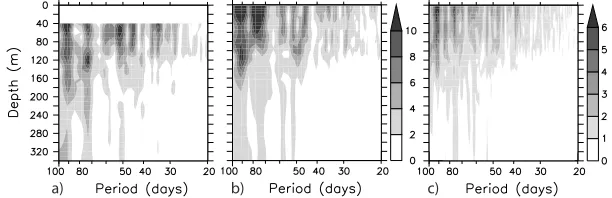
[13] To examine a dominant period of intraseasonal variations in the equatorial Indian Ocean, spectral analysis has been performed on the observed and model zonal currents at 90°E on the equator. The observed zonal currents above 400 m were obtained from ADCP mooring deployed at (0°N, 90°E) from November 2000 to December 2003 [Masumoto et al., 2005]. Figures 1a and 1b show variance spectra of the observed and model zonal currents for 2001 – 2003. Although the spectra show intraseasonal variations with a period of about 30 – 60 days, the dominance of 70 – 100-day variations is obvious in both observation and model. The intraseasonal variability within this frequency band is most prominent in the upper 100 m depth. These spectral peaks also appear in 14-year (1990 – 2003) model zonal currents (Figure 1c). Previous studies have shown that the instraseasonal variations in the equatorial Indian Ocean within this frequency band are primarily driven by winds [Han et al., 2001;Han, 2005;Fu, 2007]. In particular,Han [2005] and Fu [2007] have shown that the resonance mechanism ofCane and Moore[1981] involving the second baroclinic mode enhances the directly forced response of the 90-day variations.
Figure 1. Variance-preserving spectra of (a) observed and (b) model zonal currents at (0°N, 90°E) calculated based on 3-year record (2001 – 2003). (c) Same as in Figure 1b except calculated based on 14-year record (1990 – 2003). Note that the scale changes for Figure 1c.
[14] Given the dominance of 70 – 100-day variations, we will focus on this frequency band in the remainder of this paper. We used a band-pass filter of complex Morlet wavelet transform [Torrence and Compo, 1998] with
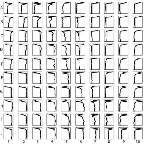
periods). The 10 10 SOM array for the model zonal current in the upper 1000 m depth is shown in Figure 2. Each node in the SOM array represents a typical vertical structure of the zonal current within the original data. In the upper-right and lower-left corners, we observe the first baroclinic mode-like structure, whereas the upper-left and lower-right corners are populated by the second baroclinic mode-like structure. The higher modes are distributed in the center.
[16] To examine the interannual modulation of the intra-seasonal variations, we have calculated a hit-repartition map for each annual cycle from April through March of the following year by calculating the number of days mapped to each node in the SOM array (Figure 3). The definition of the annual cycle is designed to capture the co-occurrence of the IOD and El Nin˜o.
[17] It is shown that during the positive IOD event in 1994 and the weak positive IOD event in 1991, the first baroclinic mode-like structure disappears in the hit reparti-tion map, while the second and higher modes are frequently seen. This indicates that the intraseasonal variations during these events are mostly dominated by the second and higher Figure 2. A 10 10 SOM array of the 70 – 100 days
band-passed model zonal current in the upper 1000 m depth at (0°N, 90°E). The vertical lines indicate the zero line.
order modes. The first baroclinic mode-like structure is still present during the 1997 positive IOD event, even though the second and higher baroclinic mode-like structures dom-inate. The inclusion of the spring Yoshida-Wyrtki jet, which involves the first baroclinic mode, is the cause of this difference as the spring Yoshida-Wyrtki jet was very weak during the 1994 positive IOD event (Vinayachandran et al., 1999).
[18] During the strong 1998 – 1999 negative IOD events, on the other hand, the first baroclinic mode-like structure dominates the variations. The hit repartition map shows more hits in the lower-left and upper-right corners. The dominance of the first baroclinic mode-like structure is also prominent during the 1996 negative IOD event. We note that the second baroclinic mode-like structure also frequently appears during the 1996 negative IOD event.
[19] These results suggest that the IOD events can have a significant impact on the dominant modes involved in the intraseasonal zonal currents in the eastern equatorial Indian Ocean. During the positive IOD events, the second and higher baroclinic mode-like structures dominate the vari-ability, whereas the first two baroclinic mode-like structures tend to dominate the variability during the negative IOD events.
5. Discussion and Conclusions
[20] The change in the dominant mode of intraseasonal variations during the IOD events may be attributed to the change in the background stratification. To check this hypothesis, we have analyzed the projection of the wind stress onto the vertical modes in term of a wind-projection coefficient [Gill, 1982],
whereHmixis the depth of the mixed layer, D is the depth of the ocean bottom, and yn(z) are the eigenfunctions of the solutions for the equations of motion.
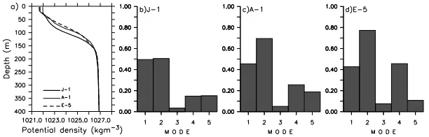
[21] The calculation of wind-projection coefficient is based on the composite density profiles of three different nodes in the SOM array:J-1,A-1, andE-5, which represent the first-, second- and higher-mode like structure, respec-tively (Figure 2). The vertical profiles of the density at (0°N, 90°E) for those three nodes are shown in Figure 4a and the
wind-projection coefficients of the first five baroclinic modes for each density profile are shown in Figures 4b – 4d. [22] As expected, there are significant variations in the wind-projection coefficients associated with the change in vertical density profiles. The J-1 pattern shows a deep-pycnocline structure, and the first two baroclinic modes are more preferentially forced (Figure 4b). When the pycno-cline becomes sharper as shown in theA-1andE-5patterns, the higher modes, i.e. the second and fourth modes, are more efficiently excited (Figures 4c and 4d). Thus, we propose that an apparent shoaling of pycnocline accompa-nied by a substantial increase of vertical stratification in the upper layer of the eastern equatorial Indian Ocean during the positive IOD events traps the wind forcing in a thin surface mixed-layer, allowing the wind forcing to project more preferentially onto the higher modes.
[23] In this study, we show that the use of the SOM to identify characteristics of intraseasonal zonal currents rep-resents a dynamic approach compatible with that of the normal mode analysis. Compared with the normal mode analysis, the SOM does not require a complete vertical profile from surface down to the bottom which is difficult to obtain from direct observation. In addition, the SOM is also able to handle missing data, where it is quite useful for data from direct observation that often contains missing values.
[24] Acknowledgments. We thank H. Sasaki for the OFES output. The present research is supported by Grant-in-Aid for Scientific Research (A) from the Japan Society for Promotion of Science for the last author. The first author is grateful for the support received from Japan Society for the Promotion of Science through the postdoctoral fellowships for foreign researchers.
References
Cane, M., and D. W. Moore (1981), A note on low-frequency equatorial basin modes,J. Phys. Oceanogr.,11, 1578 – 1584.
Fu, L.-L. (2007), Intraseasonal variability of the equatorial Indian Ocean observed from sea surface height, wind and temperature data,J. Phys. Oceanogr.,37, 188 – 202.
Gill, A. E. (1982),Atmosphere-Ocean Dynamics,Int. Geophys. Ser., vol. 30, 662 pp., Academic, San Diego, Calif.
Han, W. (2005), Origin and dynamics of the 90-day and 30 – 60-day varia-tions in the equatorial Indian Ocean,J. Phys. Oceanogr.,35, 708 – 728. Han, W., J. P. McCreary, D. L. T. Anderson, and A. J. Mariano (1999), On
the dynamics of the eastward surface jets in the equatorial Indian Ocean,
J. Phys. Oceanogr.,29, 2191 – 2209.
Han, W., D. M. Lawrence, and P. J. Webster (2001), Dynamical response of equatorial Indian Ocean to intraseasonal winds: Zonal flow, Geophys. Res. Lett.,28, 4215 – 4218.
Han, W., T. Shinoda, L.-L. Fu, and J. P. McCreary (2006), Impact of atmo-spheric intraseasonal oscillations on the Indian Ocean Dipole during the 1990s,J. Phys. Oceanogr.,36, 670 – 690.
on the West Florida Shelf using growing hierarchical the self-organizing maps,J. Atmos. Oceanic Technol.,23, 325 – 338.
Masumoto, Y., et al. (2004), A fifty-year eddy-resolving simulation of the world ocean—Preliminary outcomes of OFES (OGCM for the Earth Simulator),J. Earth Simulator,1, 35 – 56.
Masumoto, Y., H. Hase, Y. Kuroda, H. Matsuura, and K. Takeuchi (2005), Intraseasonal variability in the upper layer currents observed in the east-ern equatorial Indian Ocean, Geophys. Res. Lett., 32, L02607, doi:10.1029/2004GL021896.
Murtugudde, R., J. P. McCreary, and A. J. Busalacchi (2000), Oceanic processes associated with anomalous events in the Indian Ocean with relevance to 1997 – 1998,J. Geophys. Res.,105, 3295 – 3306. O’Brien, J. J., and H. E. Hurlburt (1974), Equatorial jet in the Indian Ocean:
Theory,Science,184, 1075 – 1077.
Pacanowski, R. C., and S. M. Griffies (1999), The MOM 3 manual,Tech. Rep. 4, 680 pp, Geophys. Fluid Dyn. Lab. Ocean Group, Princeton, N. J.
Vinayachandran, P. N., N. H. Saji, and T. Yamagata (1999), Response of the equatorial Indian Ocean to an unusual wind event during 1994,Geophys. Res. Lett.,26, 1613 – 1616.
Webster, P. J., A. M. Moore, J. P. Loschnigg, and R. R. Leben (1999), Coupled ocean-atmosphere dynamics in the Indian Ocean during 1997 – 1998,Nature,401, 356 – 360.
Wyrtki, K. (1973), An equatorial jet in the Indian Ocean,Science, 181, 262 – 264.
I. Iskandar, Institute of Observational Research for Global Change, Japan Agency for Marine-Earth Science and Technology, 2-15, Natshima-cho, Yokosuka, Kanagawa 237-0061, Japan.