Geographically Weighted Regression Model for Poverty Analysis in
Jambi Province
Inti Pertiwi Nashwari, Ernan Rustiadi, Hermanto Siregar, and Bambang Juanda
Received: 08 04 2016 / Accepted: 24 08 2016 / Published online: 30 06 2017 © 2017 Faculty of Geography UGM and he Indonesian Geographers Association
Abstract Agriculture sector has an important contribution to food security in Indonesia, but it also huge contribution to the number of poverty, especially in rural area. Studies using a global model might not be suicient to pinpoint the fac-tors having most impact on poverty due to spatial diferences. herefore, a Geographically Weighted Regression (GWR) was used to analyze the factors inluencing the poverty among food crops famers. Jambi Province is selected because have high number of poverty in rural area and the lowest farmer exchange term in Indonesia. he GWR was better than the global model, based on high value of R2, lowers AIC and MSE and Leung test. Location in upland area and road system had more inluence to the poverty in the western-southern. Rainfall was signiicantly inluence in eastern. he efect of each factor, however, was not generic, since the parameter estimate might have a positive or negative value.
Abstrak Sektor pertanian memiliki peran penting terhadap ketahanan pangan di Indonesia, tetapi juga memberi pengaruh
pada angka kemiskinan khususnya di wilayah pedesaan. Penelitian dengan menggunakan model global kemungkinan tidak sesuai lagi untuk mengetahui faktor-faktor yang mempengaruhi kemiskinan berdasarkan karakteristik spasial. Oleh karena itu, penelitian ini menggunakan metode Geographically Weighted Regression (GWR) untuk menganalisis faktor yang mempengaruhi kemiskinan petani tanaman pangan. Propinsi Jambi digunakan sebagai lokasi penelitian karena wilayah ini memiliki kemiskinan di pedesaan yang tinggi dan Nilai Tukar Petani (NTP) yang paling rendah di Indonesia. GWR memberikan hasil yang lebih baik dibandingkan model global berdasarkan nilai R2 yang tinggi, nilai AIC dan MSE yang kecil, dan uji Leung. Wilayah lereng/gunung dan jaringan jalan lebih signiikan terhadap kemiskinan di wilayah barat-selatan Jambi. Curah hujan signiikan di wilayah timur. Pengaruh setiap faktor tidak sama di setiap lokasi, karena estimasi parameter dapat positif atau negatif.
Keywords: food crop farmer, Geographically Weighted Regression, poverty, spatial analysis
Kata kunci: analisis spasial, Geographically Weighted Regression, kemiskinan, petani tanaman pangan
1.Introduction
he Asian Development Bank [ADB, 2009] reported that 82 percent of poor workers lived in rural area. Of all poor workers in rural area, 66 percent worked in non-formal agricultural sector and the remaining 46 percent worked in formal sector. Although agriculture sector plays an important role in maintaining supply for food and industrial sectors and therefore contributes to food security, the growth of agricultural sector is stagnant and is lagging behind the growth of non-agricultural sector. It is then not surprising when the poverty in rural area increased from 13.76 percent in September 2014 to 14.09 percent in September 2015 [BPS, 2016]. Moreover, the agriculture sector still contributed to the high number of poverty in rural area as indicated by the high number of poor rural area’s residents, who depended on the agricultural sector. Poverty in Indonesia has been widely studied [Lisanty and Tokuda, 2015; Sudarlan et al., 2015;
Inti Pertiwi Nashwari, Ernan Rustiadi, Hermanto Siregar, and Bam-bang Juanda
Department of Regional and Rural Development Planning Science, Bogor Agricultural University
Correspondent email: [email protected]
Sudaryanto, 2009; Sumarto and de Silva, 2013; Suryahadi and Hadiwidjaja, 2011; Teguh and Nurkholis, 2011; Warr, 2013; Yosnofrizal, 2011] to pinpoint the factors afecting poverty. However, the poverty analysis in Indonesia was previously based on the global approach, which might not be suitable considering the diferent typology and geographical locations of Indonesian islands. In other countries, the spatial approach was already applied for poverty analysis [Yamauchi et al., 2010; Smajgl and Bohensky, 2013]. Although the spatial approach was already known in Indonesia, it was used for other purposes than poverty analysis [Saefuddin, et al., 2011; Bekti and Sutikno, 2011; Saefuddin, et al., 2012]. Using diferent spatial approach, Jajang [2014] used a dynamic spatial panel model and Pasaribu [2015] used a Spatial Lag Model (SLM), Spatial Error Model (SEM) and Spatial Autoregressive Moving Average (SARMA) to analyze poverty in Indonesia.
he spatial approach does not relate only to distance, location and situation, access, correlation and pattern [Muta’ali, 2012], but also to spatial pattern, correlation between variables, and spatial process. Most of the poverty cases in Indonesia are spatially concentrated. hey are oten found in remote area,
Indonesian Journal of Geography Vol. 49, No.1, June 2017 (42 - 50)
characterized by having poor access and are located in diicult geographical location [Minot et al., 2006]. Moreover, the spatial econometrics has a correlation with regional cases and rural economic, which are based on biological and geological phenomenon, and regional science [Anselin, 1988]. A previous study [World Bank, 2007] suggested that geographical location has correlation with poverty. herefore, an analysis using geographical disaggregation technique at the lowest level of governmental structure is needed to replace the macro approach for poverty analysis in Indonesia.
In this study, the global and spatial approaches were compared and the most factors inluencing poverty were suggested. hree diferent factors, namely road system (asphalt/concrete road), location in upland area (mountain top/slope) and the amount of rainfall, are selected for the independent variables to explain the poverty cases in rural area. Diferent characteristics of each location, such as access to market or inner area, typology and climate, have impact on the poverty of food crops farmer. he upland area, which is located far and has poor accessibility to inner area, might have a high number of poverty cases; while the area with high amount of rainfall is expected to have a low number of poverty cases.
Jambi province, which is located in Sumatera Island, was used as a model for the poverty analysis using the global and spatial approach. Jambi province was selected not only because of it has high poverty cases among food crops farmers, but also has the lowest value of farmer exchange term/Nilai Tukar Petani (NTP) in Sumatera Island. he result of this study can be used as a basis to formulate strategies for poverty alleviation in Jambi province.
2. he Methods
he data obtained from 131 sub-districts in Jambi province (Figure 1) was used in current study. he independent variables used to analyze the factors inluence farmer poverty in food crops subsector were
road system, location in upland area (mountain top/ slope) and rainfall, while the dependent variable was the percentage of poor food crops farmer (Table 1). he data for dependent variable was obtained from “Pendataan Program Perlindungan Sosial”(PPLS) [BPS, 2011] and the data for independent variable was extracted from Agriculture census [BPS, 2013], the potency of rural area [BPS, 2015] and the data obtained from climatology station of Jambi Province
Global regression analysis [Hill, et al., 2011; Gujarati, 2010] (Equation 1) and Geographically Weighted Regression (GWR) (Equation 2) were used to analyze the factor(s) afecting farmer’s poverty in food crops sub-sector. he GWR model is the weighted global regression model [Fotheringham, et al., 2002, Fischer and Getis, 2010]. In this model, the model parameters are estimated for each geographical coordinate, and therefore each coordinate has diferent regression parameter estimates. In comparison to OLS or global regression analysis, the GWR model was reported as more suitable for data description [Ali, et al., 2007].
i
Where yi is dependent variable at i location (i=1,2,..,n), xik is independent variable k at i location (Table 1), β is the regression coeicient and i is the error assumed as identical, independent and has normal distribution with constant variance (α2). he assumption was tested by Kolmogorov Smirnov method for normal distribution, Glejser method for identical, and Durbin Watson method for independent. he parameters were estimated using the Ordinary Least Square (OLS) method. he GWR model is (2)
Table 1. Independent variable
Variables Deinition
Road system (Asphalt/con-crete road (X1))
he percentage of rural area based on the type of road surface of asphalt/concrete. he road connects between production center/ agricul-tural land to the main road of rural area.
Location in upland area (mountain top/slope area (X2))
he percentage of rural area located in slope or mountain top.
(
)
∑
(
)
Where (ui,vi) are the longitude and latitude coordinates at i location in certain geographical region, βk (ui,vi) is the regression coeicient k in each region or the manifestation of the continuous function of βk (ui, vi) at i location. he parameters β were estimated by Weighted Least Square (WLS) (Equation 3).
â
ˆ
(
)
(
X
W
(
)
X
)
X
W
(
)
y
Where X is the independent variable matrix, W(i) is the weighted matrix, and y is the vector of dependent variable. GWR require the weighted matrix which shows about neighboring among locations. he type of weighting matrix was kernel bi-square (Equation 4).
Where wj(ui,vi) is the weighted among location i in coordinate (ui,vi) and other location, dij is Euclidean distance i and j location, and b is bandwidth. Bandwidth is measure the distance weighting function and the extent of inluence the location to another location. Bandwidth is calculated based from Cross Validation (Equation 5),
(5)
Where
[
y
i−
y
ˆ
≠i(
b
)
]
the predicted is value from model without observation i. Identiication of spatial efect is also important to know that the data is more relevant to analyzed by spatial model, especially for GWR. he methods are Moran’s test, Local Indicator of Spatial Autocorrelation (LISA) for test of spatial independency and Breusch-Pagan test for spatial heterogeneity. Moran’s I and LISA used to determine whether there is a spatial dependency among locations with the null hypothesis is there is no spatial dependencies. Breusch-Pagan uses the null hypothesis that there is no spatial heterogeneity in the model. he models were run using R Sotware. It needs a spgwr and spdep package.3. Result and Discussion
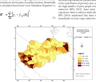
he number of poor people in rural area of Jambi province was higher than in urban area. he book of poverty data and information [BPS, 2013] revealed that around 39 percent (from 2.318.485 people) of the poor people aged above 15 years worked in agricultural sector. In 2012, around 14.33 percent of 63.529 people total agricultural workers were poor people aged above 15 years old and worked in food crops subsector. he agricultural sector in Jambi province was dominated by the subsectors of plantation and food crops. However, the food crops subsector has also been considered as one of the contributors of poverty cases, as can be seen from the high number of poor people worked in food crops subsector [BPS, 2013]. Some food crops households experience what is called as multi-dimensional poverty. BPS [2014] mentioned that there was 27.41 percent households in food crops subsector which experience
[
]
2on multidimensional poverty in 2013. his value was calculated from Multidimensional Poverty Index (MPI) which shows the composite index. It measure poverty more broadly, especially in the case of limited access to education, healthy, and quality of live. he food crops farmer household had a lower income as compared to the other type of farmer households, indicating that the welfare of food crops farmer household was also still low. Of all provinces in Sumatera Island and even in Indonesia, Jambi province had the lowest farmer’s term of trade or Nilai Tukar Petani (NTP) in 2013 [BPS, 2015]. In addition, the agricultural land owned by this type of farmer household also decreased from 1,028.41 m2 in 2003 to 963.16 m2 in 2013 [BPS, 2013], reducing the amount of crops and inally the total income received by food crops farmer. he percentage of poor food crops farmer households in Jambi province is presented in Figure 2. Most of the poor households were found in Merangin and Kerinci regencies and in the eastern part of Jambi province, such as in Tanjung Jabung Timur Regency. he distance to the regency capital seemed to have a correlation with poverty. For example, the sub-districts having the highest number of poor household, such as Sungai Tenang, Sungai Manau, and Pangkalan Jambu, are located far from Bangko, the capital of Merangin Regency. he centre of growth is a geographical location
for all activities, including economic activities [Cappelo, 2007]. herefore, the area, which are located far from the centre of growth (capital area) and has low accessibility to good infrastructure facility, might be less developed and has more poor inhabitant than area close to the centre of growth and/or with good infrastructure facility.
he poverty characteristic as function of road system, location in upland area and the amount of rainfall in each sub-district in Jambi Province varied (Figure 3). he secondary data collected from BPS [2015] showed that less than 50 percent of villages in sub-districs with high percentage of poor households had access to asphalt/concrete road from production centre to the centre of the village, conirming the connection between poverty and road system. However, interestingly high number of poor household was also found in sub-districts with good infrastructure facilities. In this case, the transport system, which connects a sub-district with other sub-districts or regencies, is lacking and the good road access was meant for other purposes, such as access for forest industry rather than for agriculture. Similarly to road system, location in upland area also contributed to the high number of poverty. A high number of poor households was found in upland area (mountain top/slope), but some were also found in lowland area, where the access to road system is considered better than in upland area. he
distance to the center of growth might be the reason for the high poverty rate in lowland area since most of the poor households in lowland area live near the shoreline/coastal area. Moreover, low poverty rate was found in the area with high amount of rainfall per year, which might be correlated to the high amount of yields. However as road system and location in upland area, the efect of rainfall on the number of poverty was not conclusive since high poverty rate was also found in the area having high amount of rainfall per year. Although having a high amount of rainfall per year, this area might be located in upland area, far from the center of economic or having poor access to the road system, which inluence their access to the center of growth.
he result of the global regression model is presented in Table 2. he global regression model assumed that the parameters for all sub-districts are similar, indicating that the factors inluencing poverty in all sub-districts was also similar.
he regression coeicient in Table 2 was used in the global regression model in equation 1, resulting in Ŷ = 13.560 + 0.150 X1 + 0.324X2 – 3.062X3. he resulting model indicated that the poverty among food crops farmers had a positive correlation with road system (asphalt/concrete road) and location in upland area (mountain top/slope). When the other variables are constant, the poverty increases by 0.150 percent and 0.324 percent due to the increase in the number of villages with good road system and the increase in the number of villages in upland area by the factor of 1, respectively. On the contrary, the amount of rainfall had a negative correlation to the number of poverty. he number of poverty decreases by 3.062 percent when the amount of rainfall increases by the factor of 1,
assuming that other variables are constant. However, the signiicant efect (p=0.05) of variables on poverty was only observed for road system and location in upland area. Furthermore, the coeicient of determination (R2) of 21.55 percent provided an indication that the poverty cases in Jambi Province could not be explained only using the global regression model and/or the three variables currently included for poverty analysis. Further residual analysis using the Kolmogorov Smirnov, Durbin Watson test and the Glejser method showed that the assumption of normal distribution and the assumption on similarity of poverty causal in all sub-districts were not met. herefore, the use of spatial modeling approach for poverty analysis in Jambi province, such as Geographically Weighted Regression, is considered. Before the spatial analysis approach was applied, the dependency analysis using Moran test and Local Indicator of Spatial Autocorrelation (LISA) and spatial heterogeneity using the Breusch-Pagan test were used to observe the spatial efect on the poverty among food crops farmers. he analysis results are shown in Table 3 and Figure 4.
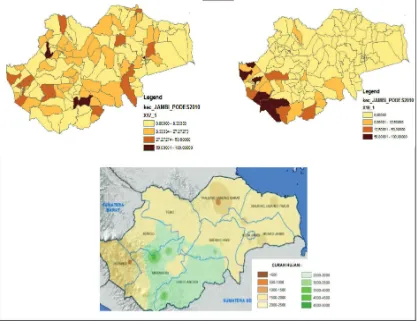
Moran index and p value were used to describe the spatial dependency. he null hypothesis (H0:I=0) means that there is no spatial autocorrelation among the sub-districts, while the alternative hypothesis (H1:I #0) means that the spatial autocorrelation among the sub-districts was observed. Based on Moran’s I analysis, autocorrelation among sub-districts was found for the variables of location in upland area, rainfall and poverty among food crops farmers (p<0.05). he spatial dependency for poverty variable indicated that the poverty among the sub-districts was correlated, especially for those in neighboring area.
he sub-districts having high number of poverty rate are close to each other, and therefore form a cluster (Figure 2), as also indicated by Moran Index of 0.457. Furthermore, the spatial dependency analysis using Local Indicator of Spatial Autocorrelation (LISA) identiies the local spatial autocorrelation or the spatial efect for each sub-district about poverty among food crops farmers. Stronger correlation among sub-districts is indicated by the low value of p. he p value in the western-southern parts of Jambi province, around Kerinci and Merangin Regencies, was lower than that in other regencies, indicating the poverty correlation among the sub-districts in Kerinci and Merangin Regencies (Figure 4). he spatial heterogeneity analysis was used to determine the spatial efect and the characteristic heterogeneity among sub-districts. Using the Breusch-Pagan test, spatial heterogeneity was found when the global regression model (Equation 1 and Table 2) was used. Also, test of the residual assumption found the residual heterogeneity. Because spatial dependency and heterogeneity efects were reported from those analyses, the use of Geographically Weighted Regression (GWR) model in equation 2 is recommended. he result of the GWR model is presented in Table 4. his model used a ixed kernel bi-square for weighting
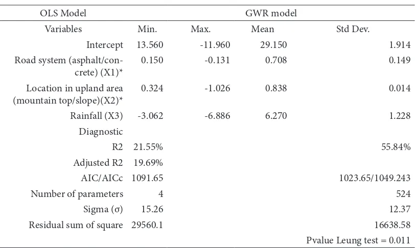
process and a bandwidth value of 0.4275. he bandwidth value of 0.4275 indicated that a sub-district will have a strong correlation with the other sub-districts in the radius of 0.4275o or 47.59 km. he estimated parameters of GWR model for each sub-district are shown in Figure 5. he regression coeicient parameter of road system can have a positive or negative value, meaning that the road system has positive or negative impact on the poverty rate (Figure 5a). he western-southern part of Jambi province had a high positive parameter estimate. his high positive value suggested that the more villages have a good road system, the higher the poverty rate is in that area. On the contrary, the increase in the number of villages with good road system contributed to the decrease in poverty rate in eastern part of Jambi. Similarly to the road system, location in upland area and the amount of rainfall also contributed to the positive and negative efects on the poverty rate.
Most of the western-southern of Jambi province, which is located in the upland area, have positive parameters value, meaning that the poverty is higher when more villages in the sub-districts are located in upland area. he efort to open a new potential and productive area is hindered by the lack of connection to the interregional road. he challenge to open the Table 4. Parameter Estimates of GWR
Variables Minimum Median Maximum
Constant -11.960 -1.986 29.150
Road system of asphalt/concrete -0.131 0.080 0.708
Location in upland area (mountain top/slope) -1.026 0.049 0.838
Rainfall -6.886 1.101 6.270
Table 5. he Comparison of GWR and Global Regression Model
OLS Model GWR model
Variables Min. Max. Mean Std Dev.
Intercept 13.560 -11.960 29.150 1.914
Road system (asphalt/con-crete) (X1)*
0.150 -0.131 0.708 0.149
Location in upland area (mountain top/slope)(X2)*
0.324 -1.026 0.838 0.014
Rainfall (X3) -3.062 -6.886 6.270 1.228
Diagnostic
R2 21.55% 55.84%
Adjusted R2 19.69%
AIC/AICc 1091.65 1023.65/1049.243
Number of parameters 4 524
Sigma (σ) 15.26 12.37
Residual sum of square 29560.1 16638.58
connection is not only due to the budget availability, but also due to the diicult location, which inluence the implementation of infrastructure program and its maintenance. Moreover, although the upland area has suitable climate and suicient natural resources for agriculture production, it is not suitable for food crops production and is prone to landslide and volcanic eruption. Diferent situation was observed for the sub-districts in the eastern part of Jambi, which is much closer to the city center than the western-southern part of Jambi. In this area, the potency for food crops production is high and most of the inhabitants work as farmer. he variable of location in upland area was not signiicantly inluence the poverty in this area, because most of the area was dominated by lowland agriculture area with irrigation system. It is then not surprising when the percentage of poverty in this area was a bit smaller than in western-southern part of Jambi. he amount of rainfall had diferent impact in diferent sub-districts. he variable of rainfall had a negative efect in the western-southern part of Jambi province and a positive impact in the central to eastern part of Jambi. Having a negative efect means that the area with high rainfall will have a lower percentage of poverty, whereas the positive value indicate that the higher amount of rainfall will contribute to the higher percentage of poverty in Jambi. his is because the high rainfall can lead to loods damaging crops. As in the Kerinci, Merangin, Muaro Jambi and Jambi City experienced frequent looding result in reduced production of rice. Similar situation was also observed in Vietnam, when higher rainfall contributed to the decrease in poverty in some areas, but increased the poverty in the other areas [Minot et al., 2006]. However, the efect of rainfall on poverty in Jambi was
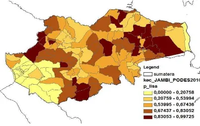
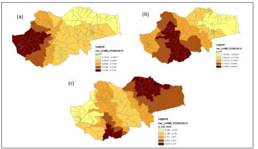
only signiicant for fewer numbers of sub-districts. he p values of each variable from the GWR model are presented in Figure 6. he variables of road system, location in upland area and the amount of rainfall have more inluence in a sub-district with low p value than in sub-district with high p value. In general, the road system had high inluence on poverty in the sub-districts of western and southern part of Jambi, while rainfall has signiicant efect on poverty for the sub-districts in the eastern part of Jambi.
Figure 6.he p value of each variable in GWR model: (a) road system, (b) upland area, (c) rain fall
a good road system, the less number of poverty will be found. Although the road system between the center of production and the center of growth in that area was good, the interregional road system might not be suicient and was far from the capital center. his poor access might be the reason for farmer’s diiculty to sell their crops and to obtain the production input, increasing the number of poor people in the area with a good local road system. Furthermore, the concentrated economic activity might not be able to reduce the poverty rate in those areas. Because the commodity price was lower than the consumer price, farmer’s income was lower than their expenditure. Consequently, the farmer exchange value (NTP) was lower, causing the increase in the number of poverty. In this case, the center of economic in such area failed to contribute to the positive spillover impact (spread efect) to its hinterland.
Based on the global regression analysis, variables afecting the poverty among food crops farmers were road system (asphalt/concrete road) and location in upland area. he global regression model, however, assumed that the parameter in all locations were similar and signiicant. his assumption was diferent from the observed characteristic since road system, location in upland area and the amount of rainfall had diferent inluence on poverty rate in each location. herefore, the global regression model was less suitable for the poverty analysis, which was location dependent. Alternatively, the GWR model, which considered the spatial efect, was be used for the poverty analysis for Jambi province. his conclusion was supported among
others by the low value of the coeicient determination (R2) and higher AIC and Mean Square Error (MSE) as compared to GWR model (Table 5). he GWR analysis became more important considering also the dependency analysis and spatial heterogeneity. he result that GWR analysis was better than global regression model for poverty analysis in Jambi province conirm the previously described theory that spatial analysis should be used, instead of global regression model, for poverty analysis when spatial heterogeneity is observed. he better performance of GWR model over a more global model was also reported by Kam et al. (2005), Ali et al. [2007], Deller [2010], and Ali hongdara et al. [2012].
5.Conclusion
of poverty the area might also be high. Similarly, when the area was in lowland area, but the poverty is high, the area was probably located far from the center of growth, preventing fast access of agricultural product to the central market. However, those three variables were only able to explain around 50% of the poverty occurrence in Jambi sub district. herefore, analysis which included other variables might be of interest.
Acknowledgement
hank you for Ministry of Agriculture which has funded this reseach through the scholarship program.
References
ADB (2009). Kesejahteraan Petani dan Pengentasan Kemiskinan [internet]. [diacu 2015 Oktober 24]. http://www.mediaindonesia.com/mipagi/ r e a d / 1 6 5 2 1 / K e s e j a h t e r a a n P e t a n i d a n -Pengentasan-Kemiskinan (in bahasa indonesia). Anselin, L. (2013). Spatial econometrics: methods and
models (Vol. 4). Springer Science & Business Media. Ali, K., Partridge, M. D., & Olfert, M. R. (2007). Can
geographically weighted regressions improve regional analysis and policy making?. International Regional Science Review, 30(3), 300-329. Badan Pusat Statistik (2013). Laporan Hasil Sensus
Pertanian 2013 (Pencacahan Lengkap), BPS Provinsi Jambi, Jakarta. (in bahasa Indonesia). Badan Pusat Statistik (2014). Analisis Sosial Ekonomi Petani
di Indonesia. Hasil Survei Pendapatan Rumah Tangga Usaha Pertanian. Sensus Pertanian 2013, BPS, Jakarta. Badan Pusat Statistik (2015). Statistik Potensi Desa Provinsi
Jambi 2014, BPS, Jambi. (in bahasa Indonesia). Badan Pusat Statistik (2015). Indeks Harga yang Diterima
Petani (It), Indeks Harga yang Dibayar Petani (Ib), dan Nilai Tukar Petani (NTP) Menurut Provinsi, 2008-2014 [internet]. [diacu 2015 Mei 25]. Tersedia di http://bps. go.id/linkTabelStatis/view/id/1482.(in bahasa Indonesia). Badan Pusat Statistik (2016). Proil Kemiskinan Indonesia
September 2015, BPS, Jakarta.(in bahasa Indonesia). Bekti, R.D., and Sutikno (2012). Spatial durbin model to identify inluential factors of diarrhea. J. Math. Statistics, 8: 396-402 Brunsdon, C., Fotheringham, A. S., & Charlton,
M. (2002). Geographically weighted summary statistics—a framework for localised exploratory data analysis. Computers, Environment and Urban Systems, 26(6), 501-524. Cappelo, R (2009). Spatial Spillover and Regional Growth : a
Cognitive Approach. European Planning Studies, 17(5) Fischer, M.M., and Getis, A (2010). Handbook
of Applied Spatial Analysis, Sotware Tools, Methods and Applications, Springer, New York. Fotheringham, A. S., Charlton, M. E., & Brunsdon, C. (1998). Geographically weighted regression: a natural evolution of the expansion method for spatial data analysis. Environment and planning A, 30(11), 1905-1927. Gujarati, D.N (2010). Basic Econometrics.
Mc Graw-hill Companies, New York. Hill, R. C., Griiths, W. E., and Lim, G. C (2011). Principles
of econometrics, John Wiley & Sons, Inc, USA. Jajang (2014). Modiikasi Statistik Getis Lokal pada
MatriksPembobot AMOEBA untuk Model Panel Spasial dan Kajian Performanya. Sekolah Pascasarjana IPB, Bogor.
Kam, S. P., Hossain, M., Bose, M. L., & Villano, L. S. (2005). Spatial patterns of rural poverty and their relationship with welfare-inluencing factors in Bangladesh. Food Policy, 30(5), 551-567. Lisanty, N., & Tokuda, H. (2015). Comprehending Poverty
in Rural Indonesia: An In-depth Look inside Paddy Farmer Household in Marginal Land Area of Banyuasin District, South Sumatra Province. International Journal of Social Science Studies, 3(3), 129-137. Minot, N., Baulch, B., & Epprecht, M. (2006). Poverty
and inequality in Vietnam: Spatial patterns and geographic determinants (p. 148). Washington, DC: International Food Policy Research Institute. Muta’ali (2012). Daya Dukung Lingkungan Untuk
Perencanaan Pengembangan Wilayah. Badan Penerbit Fakultas Geograi, Universitas Gadjah Mada Pasaribu, E (2015). Dampak Spillover dan Multipolaritas
Pengembangan Wilayah Pusat-Pusat Pertumbuhan di Kalimantan. Sekolah Pascasarjana. IPB. Saefuddin, A., Setiabudi, N. A., & Achsani, N. A. (2011).
On comparison between ordinary linear regression and geographically weighted regression: With application to Indonesian poverty data. European Journal of Scientiic Research, 57(2), 275-285. Saefuddin, A., Setiabudi, N. A., & Fitrianto, A. (2012).
On comparison between logistic regression and geographically weighted logistic regression: With application to Indonesian poverty data. World Applied Sciences Journal, 19(2), 205-210. Smajgl, A., & Bohensky, E. (2013). Behaviour and space in agent-based modelling: poverty patterns in East Kalimantan, Indonesia. Environmental modelling & sotware, 45, 8-14. Sudarlan, R.I., and Yusuf, AA (2015). Impact Of Mining
Sector To Poverty And Income Inequality In Indonesia: A Panel Data Analysis, International Journal Of Scientiic & Technology Research, 4 (06) : 195-200. Sudaryanto, T., Susilowati, S. H., & Sumaryanto, S. (2009).
Increasing Number of Small Farms in Indonesia: Causes and Consequences. In European Association of Agricultural Economists, 111th Seminar. Sumarto, S, and de Silva, I (2013). Poverty-growth-Inequality Triangle: he Case of Indonesia (No. 57135), University Library of Munich, Germany. Suryahadi, A., & Hadiwidjaja, G. (2011). he
role of agriculture in poverty reduction in Indonesia. Jakarta: SMERU Research Institute. Teguh, D., & Nurkholis, N. (2011). Finding out of the
Determinants of Poverty Dynamics in Indonesia: Evidence from Panel Data (No. 41185). University Library hongdara, R., Samarakoon, L., Shrestha, R. P., &
Ranamukhaarachchi, S. L. (2012). Using GIS and spatial statistics to target poverty and improve poverty alleviation programs: A case study in northeast hailand. Applied Spatial Analysis and Policy, 5(2), 157-182. Warr, P (2013). Food Security, Agriculture, and Poverty in Asia. World Bank (2007). Era Baru Dalam Pengentasan Kemiskinan
di Indonesia. Indopov. he World Bank. Jakarta Yamauchi, F., and Muto, M. S, Chowdhury, R. Dewina,
and S. Sumaryanto (2010). Are Schooling and Roads Complementary? Evidence from Rural Indonesia. JICA Research Institute Working Paper, 10 Yosnofrizal (2015). Petani dan Jerat Kemiskinan