Spatio-Temporal Deforestation Measurement Using
Automatic Clustering
Irene Erlyn Wina Rachmawan, Ali Ridho Barakbah, Tri Harsono
Information dan Computer Engineering deforestation rate in Indonesia reached 0.84 million hectares, exceeding Brazil. According to the 2009 Guinness World Records, Indonesia's deforestation rate was 1.8 million hectares per year between 2000 and 2005. An interesting view is the fact that Indonesia government denied the deforestation rate in those years and said that the rate was only 1.08 million hectares per year in 2000 and 2005. The different problem is on the technique how to deal with the deforestation rate. In this paper, we proposed a new approach for automatically identifying the deforestation area and measuring the deforestation rate. This approach involves differential image processing for detecting Spatio-temporal nature changes of deforestation. It consists series of important features extracted from multiband satellite images which are considered as the dataset of the research. These data are proceeded through the following stages: (1) Automatic clustering for multiband satellite images, (2) Reinforcement Programming to optimize K-Means clustering, (3) Automatic interpretation for deforestation areas, and (4) Deforestation measurement adjusting with elevation of the satellite. For experimental study, we applied our proposed approach to analyze and measure the deforestation in Mendawai, South Borneo. We utilized Landsat 7 to obtain the multiband images for that area from the year 2001 to 2013. Our proposed approach is able to identify the deforestation area and measure the rate. The experiment with our proposed approach made a temporal measurement for the area and showed the increasing deforestation size of the area 1.80 hectares during those years.
1. INTRODUCTION
Earth surface is covered by two typical forests, providing an amazing diversity of ecosystem and functionality. One of the forest types is tropical forests, located in the Earth’s equator providing oxygen for living things and rich ecosystems giving fundamental roles in the essential contribution to the planet. Nowadays, tropical forests of all varieties such as rainfall forests disappear rapidly due to denudation of forest landscapes by humans to make a field for farms, to harvest timber for fuel, and to build urban areas [1]. This process is known as deforestation which involves burning, logging and acts damaging the forest. The deforestation occurs over and over again in certain parts of the world, particularly in many tropical countries such as South America, Africa, and Southeast Asia. The deforestation of tropical rain forests is a serious threat of life for human beings and natures. It effects profound impacts on global climate changes and causes extinction for thousands of species on this earth. Such massive destruction of tropical forests leads to loss of natural functions like the destruction of wildlife habitats, soil erosion, and even hustles climate changes.
The annual forest loss in the Southeast Asian nation is now the highest in the world, exceeding even Brazilian Amazon. More than half of loss (3 million hectares or 51 percent) occurred in lowland forests, the most endangered of Indonesia's forest types. But forest loss in wetlands areas increased at an even faster rate, accounting for 2.6 million hectares or 43 percent of overall loss. According to a new study published in Nature Climate Change despite a high-level pledge to combat deforestation and a nationwide moratorium on new logging and plantation concessions, deforestation time to time much increasingly occurs in Indonesia [2]. The rate of deforestation in Indonesia itself exceeded Brazil Amazon, where the highest Indonesia deforestation rate occurred in Sumatra and Borneo. Borneo is an island in Indonesia that initially has a huge area of forest providing biodiversity for living things. The finding of natural research [3] shows that selectively logged forests are more likely to be cleared than old-growth forests. Forests that have been stripped of their high value timber are significantly less valuable for commercial exploitation, increasing pressure to clear them outright for industrial plantations. At this rate of deforestation, Borneo becomes one of the critical areas that have big deforestation acts year by year.
satellite and it can be used to analyze nature changes such as deforestation area. The multispectral images from Landsat satellite are composed of seven bands or layers, and each band represents a different portion of the electromagnetic spectrum which means each spectrum has different information.
This paper proposes a new approach for detecting deforestation area using Multispectral image by combining image processing and unsupervised classification methods or clustering. Current research about multispectral classification algorithms has gained attention in these recent days, due to their good performance in showing desired information from multispectral images. To produce groups of similar object and generate a new image of clustered image, the clustering algorithm is applied to specify and identify a new cluster of Multispectral images with a high degree of similarity toward aims to clearly detect deforestation area and give a brief number of existing areas in Multispectral images captured for one period of time. Therefore, this paper proposes a new approach for detecting deforestation area from multispectral images by using Automatic Clustering. It groups a correct cluster area automatically by considering the color features of multiband images. The result of Automatic Clustering is the number of distinct areas could have been existing in one period of time. The result from Automatic Clustering will be processed with clustering algorithm in order to produce a new map that correctly separate the deforestation area and forest area. The algorithm used for clustering algorithm is K-Means algorithm, which known as one of the common methods for clustering big data size [4]. The simplicity of K-Means made this algorithm can be implemented in various cases dealing with big data size. K-Means algorithm is a clustering method that separates data into k groups. K-Means algorithm is popular to be implemented for clustering huge and large data size quickly and efficiently. However, K-Means is very sensitive in initially generated centroids. Because of initial centroids generated randomly, K-Means does not always guarantee the optimal clustering result. In some case K-Means algorithm will not reach global optimum. Therefore, this paper uses Reinforcement Programming [5] to optimize initial centroids for K-Means.
2. RELATED WORKS
Many approaches have been proposed for mining the temporal association patterns, such as cyclic association rules, periodic association tules and calendric association rules. C. Immaculate Mary and S.V. Kasmir Raja [6] presented ant colony as optimization for K-Means. Stolorz et. al. [7] presented spatio-temporal data analysis and provided queries for geographical patterns such as cyclones, hurricanes, and fronts.
Some researchers are interested in mining Spatio-temporal patterns in earth science data, where they apply existing data mining techniques to find clusters and to analyze the difference of spatial-data. Setia Darmawan [8] presented identification of deforestation area using MODIS EVI 250 m in 2000 and 2012 to identify deforestation rate in Java island. MODIS EVI is one of kind MODIS image which is able to detect vegetation based on photosynthesis rate and vegetation density using Fuzzy C-Means with 13 numbers of clusters. Sheng Zheng et. al. [9] made research to identify deforestation using Landsat data using two methods which are simple linear regression model and curve model. Pickup and Foran [10] developed a method to monitor landscapes for pastoralism based on the spatial variability of the vegetation. The spatial autocorrelation function and mean-variance plots of a spectral indicator were found to be successful in discriminating between the cover responses for typical of good and poor rainfall years. For drought conditions, the decrease in spatial autocorrelation with increasing spatial lag is rapid since the ground surface is bare and most of the vegetation signals come from scattered areas of trees and shrubs. A low decay rate of the autocorrelation function indicated a greater spatial uniformity of the landscape, e.g. during wet periods, when more ground cover, reduces the contrast between the bare soil signal and others produced by trees and shrubs. Similar observations were made by Lambin [11] over the seasonal and inter-annual cycle of three West African landscapes. Vogt [12] also analyzed the seasonal changes in spatial structure of a West African vegetational landscape, showing that there is a marked seasonal cycle in the spatial structure of a vegetation index (NDVI), and that zones of ecological transition have an identifiable seasonal dynamic in spatial structure. However, the monitoring of these spatial variability measures only provided for a qualitative description of the cover state.
3. ORIGINALITY
will be calculated by a simple differential process to indicate the change of deforestation area in temporal time, and calculate the deforestation area by counting pixels of clustered area which has deforestation area as a label and multiply by satellite scale.
4. SYSTEM DESIGN
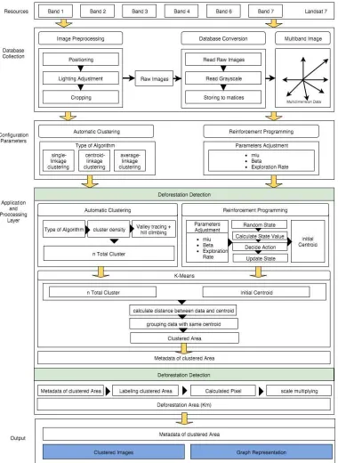
The proposed system consists of 5 phases: (1) Collecting data resources, (2) Database Collection, (3) Configuration Parameters, (4) Application and Processing Layer and (5) Output Representation. The whole system design is shown in Figure. 1.
4.1. Collecting data resources
The proposed system using real satellite image data from Landsat satellite, the services used in this system is Landsat 7 with total dataset consist of 6 bands. From Band 1, Band 2, Band 3, Band 4, Band 5 and Band 7, where each band contains 2000 x 2300 pixels.
4.2. Database Collection
Database collection is the process to reverse the data satellite into database format. This process has two segments, the first one is image preprocessing where images going through several processes like positioning, light adjustment, and cropping to make sure the position and lighting of images are not dissimilar. After preprocessing process, raw images is created and will be ready to be converted to a database, by reading the multispectral images and storing to matrices in the database. The result of database collection is to create a multidimensional data representing multiband images.
4.3. Parameters Configuration
Figure 1. Design System of our proposed approach for deforestation measurement
4.4. Application and Processing
Generating initial centroids, (3) K-Means for multiband images clustering, (4) Clustered-Image Difference Calculation.
4.4.1. Automatic Clustering
Clustering process is a step to classify the area of deforestation to get the information from its clusters. Due to the amount of the area that will be clustered is unknown, it is difficult to cluster the area with usual clustering techniques which requires the exact number of cluster should be known. Therefore, the automatic clustering process will be used for this process where the variance will be calculated and used as the measurement to get the optimum number of cluster. This cluster variance of each moving variance is designed by the variance within cluster, and it judges having reached the global optimal solution based on this tendency [13]. From the cluster variance, finding the ideal cluster is very difficult because the minimum variance cannot directly be applied to find the global optimum as an ideal cluster. For finding the global optimum of cluster construction and avoiding the local optima, we apply our Valley Tracing method [13] to find the global optimum. First of all, patterns of the moving variance should be described and analyzed possibility of the global optimum that resides in the valley of patterns:
Vi-1>= Vi and Vi+1> Vi (1)
Where Vi is variance to i, for i=1..n, and n is latest stages of cluster construction.
Figure 2. Different value of altitude
Then, identify the different value of altitude ∂ for each stage.
∂ = (Vi+1 – Vi) + (Vi-1 – Vi)
= (Vi+1 + Vi-1) – (2 x Vi) (2)
The global optimum can be obtained from the maximum value of ∂. Accuracy of the valley tracing method can be acquired by defining:
(3)
4.4.2 Reinforcement Programming for Generating Initial Centroids In this phase, a new approach to generating initial centroids for Means is stated, by using Reinforcement Programming, for optimizing K-Means by modifying Reinforcement Learning to solve a function based problem. Reinforcement Programming (RP) algorithm [14] is the algorithm using basic concept of reinforcement learning. In its implementation, Reinforcement programming has the same behavior of Reinforcement Learning, RP involving a balance between exploration of uncharted territory and exploitation of current knowledge to find a solution. The solution determined by as much reward as possible in process learning. Reward and punishment are a value given by environment from the agent step.
In RP, this policy is learned through trial-and-error interactions of the agent with its environment: on each interaction step the agent senses the current states of the environment, chooses an action to perform, executes this action, altering the states of the environment, and receives a scalar reinforcement signal r (a reward or penalty). The benefit of Reinforcement Programming is to bring a benefit in optimization case using an intelligent learning approach based on Reinforcement Learning. With involving the characteristics of Reinforcement Learning, Reinforcement Programming provides an experience-based learning to achieve the global optimum.
a. Main Variables of Reinforcement Programming
Reinforcement Programming is mainly based on the Reinforcement Learning. A number of slight modifications of Reinforcement Programming can be formulated where:
- β : is a variable value to give impact to step that the agent will take
- µ : a variable that will set a step value to the last step
The goal of the agent in an RP problem is to learn an optimal solution by set action dp . step that action is accumulated from the previous step with the direction of step that will be taken. The current state will be assigned in variable newS. New state will be accumulated by current new states and action:
newSp newSp + action (3)
The RL technique is well-known uses a strategy to learn an optimal via learning of the action values. It iteratively approximates new state. In RP, the condition of exploitation or exploration are decided by random:
p is the probability of taking action whether to exploit or explore a finite state. To balance exploitation and exploration p can be set in 0.5. The variables on reinforcement Programming structure is given in Figure 3.
The initial state is the first position of agent to start solving the problem. The state can be initiated as assigned values or random numbers depending on cases that will be handled by the agent. The variable reward is an array to save reward of each state that has been declared. To change the action direction of agent we need to declare a direction variable. In first position, the direction can be assigned with a positive number to increase the direction in positive direction. The action value is an array to save calculation of the action that has been taken by the agent. The modification of different heuristic cases will change the condition of variable state and direction.
b. System Architecture
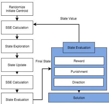
System architecture is shown in Figure 3, explaining the flow of Reinforcement Programming in order to achieve the best solution for optimizing initial centroids in K-Means. The basic Reinforcement Programming algorithm starts with an initialization phase, where:
i. Assign data item and set into variable dataset
ii. Set modeling state value calculation (depend on optimization cases) iii. Set probability for exploration rate. Use 0.5 to get a balanced action for
exploration and exploitation.
iv. Assign the value of new state in the state.
v. The agents process state evaluation to whether receiving reward or punishment for the current action.
This is done using an index that stores the positions of all ‘free’ data items on the grid. The executinal steps of RP is shown in Figure 3.
Figure 3. Executional steps of Reinforcement Programming
Centroid as the state. As for state value calculation counted from a variance of cluster homogeneity. Then RP will begin state exploration in a finite environment of the problem, the actions that can be taken by an agent is determined by exploration rate. If a random number is bigger than exploration rate than the agent will choose solution randomly in a finite area. But if the random numbers are smaller than exploration rate than agent will consider taking an action based on reward. After take an action agent updates the current state and calculates current state value. A value from current state will label as reward or punishment, and determine the next direction of exploration. If an agent receives punishment, then the agent will change its direction for the next exploration step. This process iterates in some value that already assigned as a number of learning time for the agent of RP.
An extension of this algorithm is presented where the parameter is an adaptively updated during the execution of the algorithm. This algorithm is given in Figure 4. Reinforcement Learning needs to initialize dataset to identify problem environment. Agent will place randomly or assigned value depends on handled cases. After calculating state value, an agent will determine action between exploration and exploitation. Then execute the action and calculating new state value to determine the reward based on state current value.
Reward of new state in the environment is computed through the following Eq.3 and Eq.4.
rp rp + β . (1-rp) (5)
The equation 5 shows the formula for increasing reward value.
rp rp - β . (1-rp) (6)
In case to give punishment, Reinforcement Programming used Eq.6 to decrease reward value. Where β is a constant to set a value of reward with scalar 0.1 until 1. The more scalar that will be used it will impact the increase or decrease value of the reward. The output of Reinforcement Programming algorithm is a solution to the given problem.
Let A={ai| i=1,…,f} be attributes of f-dimensional vectors and X={xi| i=1,…,N} be each data of A. The K-Means clustering separates X into k partitions called clusters M={Mi| i=1,…,k} where M ∊ X is Mi={mij| j=1,…, n(si)} as members of si, where n(si) is number of members for si. Each cluster has cluster center of C={ci | i=1,…,k}, solution of RP are represented by state S={Si | i=1,…,k}. The following execution steps of the proposed algorithm can be described as follows:
1. S Initiate its algorithm by generating random starting points of initial centroids C and describe as state S.
2. Calculate variance value (sv) of current state 3. R random a number between 0 and 1.
4. If R > exploration rate, index of state will randomly chosen 5. If R < exploration rate, index chosen will consider reward value 6. Update and calculate variance value (newsv) of new state newS (Eq.4)
7. If newsv < sv, then S newS and calculate reward (Eq.5)
Else if newsv > sv, then calculate reward with giving a punishment (Eq.6)
Else change direction
8. If i <iteration, back to Step 3.
After processing, it will generate the designated initial centroid Cp where p=1,2, ...,k. Then, we can apply it as initial centroids for K-Means clustering. The experiment result will perform the accuracy of proposed method.
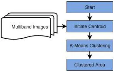
4.4.3 K-Means for multiband images clustering
In this section, the clean data from data-preprocessing function will be reads and automatically splits into clusters from the images by color information.
Figure 4: Processing flow of multispectral image clustering
leads the extraction specific geographical result area from satellite images. As for color clustering, the function divides the pixels of satellite image into specified number of groups by K-Means algorithm. K-Means algorithm works by calculating data and centroid then grouped with pixels which choose the same centroids.
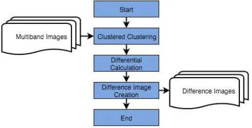
4.4.4 Clustered-Image Difference Calculation
Difference calculation function creates difference-image from the multiband image clustering result. First, from the result of clustering, the function extracts the specified colored-area for extracting difference area. Then, by comparing the extracted area between temporal images, the function will produce an increasing and decreasing area. By drawing each area by specified color, the function displays difference-images result from calculation process.
Figure 5. Processing flow of Difference Calculation
4.5. Output Representation
The last phase of this system is output representation, where the system will give two output of deforestation detection and measurement, the output presented both in images and graph.
5. EXPERIMENT AND ANALYSIS
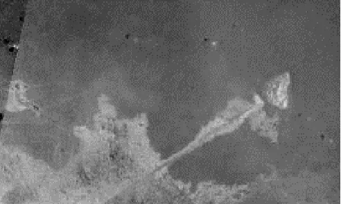
Mendawai is an area in Borneo that has noticeable deforestation activity in last 13 years. Applicating Kmeans for clustering forest and land area in Mendawai will give efficient effort for measuring deforestation area. In Mendawai, there are three clusters indicating difference nature creatures which consist of vegetation, water, and bare soil.
Using K-Means, the result will separate multiband satellite image two classes over sources data that will be clustered. The important element for analysis is vegetation area, it used for calculation function to measure forest that exists in the recent year. Fitness value of cluster will be calculated by using variance value of a cluster. Smallest number of cluster variance will show the best cluster performance.
Figure 6. An experiment area: Mendawai, Borneo, Indonesia.
This paper shows the optimum result from solving K-Means using Reinforcement Programming for optimization. The experiment has been done 100 times, and then a clustering performance of the proposed method is compared with common K-Means.
5.1.Study area
The data sets used for comparison experiments consist of 6 bands. The experiments are performed over 2D maps dataset. This dataset is clustered with K-Means to produce a clustered area. The data set samples are to be tested using Means using Reinforcement Programming and common K-Means. The use of Reinforcement programming will accelerate accuracy value of K-Means performance. In this experimental, these six bands were used as one dataset. This six dataset are composed of Band 1, Band 2, Band 3, Band 4, Band 5, and Band 7. Band 6 could not be implied as resource data, it is because band 6 showing unclear captured data. So, if we include band 6 to system,
Figure 7. Six Band of Mendawai, Borneo
Experimental Comparison
The following variance factor (V) is defined as a performance measurement in these experiments. The variance constraint [13] can express the density of the clusters with variance within cluster and variance between clusters [15]. The ideal cluster has minimum variance within clusters (Vw) to
express internal homogeneity and maximum variance between clusters (Vb)
to express external homogeneity [16].
The average error and average time are taken by the K-Means from two different algorithms will be proceeded and compared. It is used to find the best algorithm for solving multispectral images. The two algorithms that will be compared are K-Means using Reinforcement Programming and common K-Means. The following table in each algorithm will show the result and performance of each algorithm.
As for the experiment result, we ran total 100 times experiment. It shows in Table 1 and Table 2. We ran 10 times for the 10 iteration experiment and produced weak stability, 10 times for 50, 100 and 150 iterations and produced high stability for solving the problem.
A. Automatic Clustering to identify automatic cluster number of multispectral
images.
In the first step clustering process, Automatic Clustering runs right before K-Means clustering method. The main goal of using Automatic Clustering is to assign the accurate number of cluster. If Automatic clustering
Band 1 Band2
Band3 Band4
is not used, the cluster number will be assigned with a static value, and leads because Automatic Clustering is a type of hierarchal clustering methods of which they can not handle big data. The maximum arrays that can be handled by hierarchal clustering methods are 1000 arrays. So the images are resized from the satellite images into compressed the dataset.
• Collect grayscale values of each pixel in every multiband image at one cluster. This step is repeated until the optimum cluster number is found.
• Measure the Variance values from each cluster. Then, do Valley Tracing in Eq.2 to produce the optimum number of clusters.
The actual optimum number of cluster is to determine by Eq. 2 of which the value of is the global optimum of cluster number. After the implementation of the steps, the result is used as the K parameter in K-Means for clustering multispectral images.
Figure 8. Resize of Multispectral images.
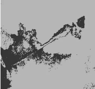
Figure 9 shows the result of automatic clustering represented in 2 color clusters: (1) green space indicating forest land, and (2) orange space indicating damage area or deforestation area. Figure 10 shows number of deforestation areas in Mendawai Borneo from 2001 until 2013. Because the number of clusters could be identified automatically using Automatic Clustering, the SSE value also can be compared to represent the validity match number for each year as shown in Figure 10. The smaller number of SSE identified the appropriate number of clusters.
using Automatic Clustering of data 2004 without Automatic Clustering of data 2004 Figure 9. The difference of a cluster member between Automatic Clustering and
manual assigning number
0 50 100 150 200 250
2 0 0 1 2 0 0 2 2 0 0 3 2 0 0 4 2 0 0 5 2 0 0 6 2 0 0 7 2 0 0 8 2 0 0 9 2 0 1 0
S
S
E
YEARS
SSEAC SSE
Figure 10. SSE value between Automatic Clustering and static assigned number of clusters
B. Optimizing K-Means to cluster Multispectral Images
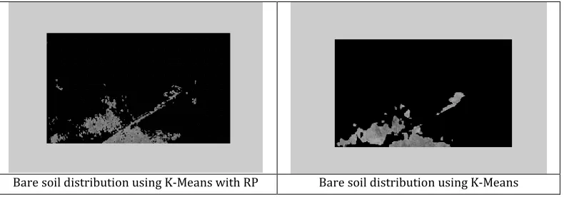
Reinforcement Programming is used to increace the accuracy of initial centroids. Figure 10 shows that Reinforcement Programming has more stable after reaching greater number of iterations. It is optimized by reinforcement programming with gaining its experience in beginning of iteration, and after reach some number of iterations, Reinforcement programming became more intelligent and can reach better solution by its own knowledge and obtain better performance to solve minimization problem. Figure 11 performs the result of identified soil distribution in Mendawai, Borneo, Indonesia. The accurate result of soil clustering can be shown using K-Means with Reinforcement Programming as K-Means optimization. Figure 12 shows complete reshaping images using K-Means with Reinforcement Programming as optimization centroid. It gave much improvement for K-Means with Reinforcement Programming rather than with random initialization, as shown in Figure 13.
Bare soil distribution using K-Means with RP Bare soil distribution using K-Means
Figure 12. Reshaping image after clustered by K-Means with RP
Figure 13: Reshaping image after clustered by common K-Means
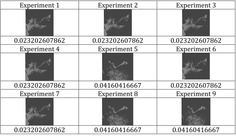
For experimental study, we did 13 times of experiment for clustering multispectral images using RP, as shown in Table 1, with a value of cluster variance in each experiment. While the experimental result for common K-Means is shown in Table 2, containing variance calculation in every experiment.
Table 1. Experimental Result of K-Means using Reinforcement Programming with overall cluster variance
Experiment 1 Experiment 2 Experiment 3
0.023202607862 0.023202607862 0.023202607862
Experiment 4 Experiment 5 Experiment 6
0.023202607862 0.04160416667 0.023202607862
Experiment 7 Experiment 8 Experiment 9
0.023202607862 0.04160416667 0.04160416667
Table 2. Experimental Result of common K-Means cluster variance
Experiment 1 Experiment 2 Experiment 3
0.08160416667 0.023202607862 0.023202607862
Experiment 4 Experiment 5 Experiment 6
0.06160416667 0.06160416667 0.023202607862
Experiment 7 Experiment 8 Experiment 9
Table 3. Performance of common K-Means and K-Means using Reinforcement Programming
Parameter Common K-Means K-Means using RP
Execution Time (min) 14 11
Average Variance 4.44906082 x 10² 2.42026078 x 10² Average Iteration for fixed centroid 4 2
As for result of comparison process, Reinforcement Programming shows a better performance to optimize Means rather than common K-Means with random initialization. The common K-K-Means shows longer computational time compared to K-Means optimized by Reinforcement Programming.
C. Deforestation Measurement
Figure 14 shows the diference extraction results after clustering proces using Reinforcement Programming. The number of clusters in study area is 2. There are 2 color clusters which are green color indicating forest area and orange colour indicating retreated area. The forest shows a minor degradation number of forests from 2000 until 2005. Starting from 2006, the number of deforestation areas dramatically increased. During 2007 until 2008, the deforestated areas still shows in Mendawai compared with a big difference between 2006 and 2007. The differences could indicate the major deforestation acts from 2006 until 2009. The number of deforestation areas started growing in late of 2009 until 2010. During 2010 until 2013, there was no change in forest area whether for reforestration or deforestation. After 2014, the area in context of deforestation has gradually decreased and at this point reforestation got successfully, though the deeper analysis with forest specialist is needed to ensure the real area of reforestation.
Figure 14 shows number of deforestation areas in Mendawai borneo from 2001 until 2013. The deforestation has gradually increased starting from 2006 to 2011. The areas calculated by counting pixel in orange space and multiplied by image scale where landsat satellite image was taken. The graphics in Figure 15 shows the trend of deforestation in Mendawai, Borneo in 2001-2013 by using Kmeans optimized by Reinforcement Programming.
2001 2002 2003
8.113 km2 40.520 km2 39.177 km2
2004 2006 2007
105.43 km2 106.39 km2 106.39 km2
2008 2009 2010
106.39 km2 165.44km2 165.44 km2
2011 2012 2013
165.44 km2 120.4 km2 101.4869 km2
Figure 14. The final result of differential extraction and image recreation (within 2 clusters where green shows the forest area and Orange shows the retreated forest
area by years).
6. CONCLUSION
This paper proposed a new approach for measuring spatio-temporal rate of the deforestation using our automatic clustering algorithm. The experiment of this research which operates big satellite data was presented by comparing the manual approach and our approach for automatic deforestation measurement with automatic clustering and K-Means optimization with our Reinforcement Programming algorithm. From the experiment, our proposed approach is able to automatically make spatio-temporal automatic deforestation measurement. This experimental study used multispectral images selected from Landsat 7 in 2001-2013 consisting of 6 bands. From series of experimental study, our proposed approach can be applicable to automatically measure the deforestation rate area. The experimental result with our proposed approach performed that the deforestation rate in Mendawai, Borneo escalates quickly from 2002 to 2011, from 50 thousand to 150 thousand hectares (300%). It indicates that our proposed approach can give a good performance for examining the feasibility, applicability and effectiveness to be applied for deforestation area detection and visualization using automatic clustering.
REFERENCES
[1] Rebecca Lindsey, Tropical Deforestation, Nasa Earth Observatory, http://earthobservatory.nasa.gov/Features/Deforestation, 2007.
[2] Rhett Butler, Mongabay Forest Lost, mongabay.com, 2015.
[3] Roberto Cazzolla Gatti, Simona Castaldi, Jeremy A. Lindsell, David A. Coomes, Marco Marchetti, Mauro Maesano, Arianna Di Paola, Francesco Paparella, Riccardo Valentini, The Impact of Selective Logging and Clearcutting on Forest Structure, Tree Diversity and Above-Ground Biomass of African Tropical Forests, Ecological Research, January 2015, Volume 30, Issue 1, pp 119–132.
[4] H. Ralambondrainy, A Conceptual Version of the K-Means Algorithm,
Pattern Recognition Letters, Volume 16, Issue 11, November 1995,
Pages 1147-1157.
[5] Irene Erlyn Wina Rachmawan, Ali Ridho Barakbah, Tri Harsono, Multiband Satellite Image Clustering using K-Means Optimization with Reinforcement Programming, The Fourth Indonesian-Japanese Conference on Knowledge Creation and Intelligent Computing (KCIC) 2015, March 24-26, 2014, Surabaya/Bali, Indonesia.
[6] C. Immaculate Mary, S. V. Kasmir Raja, Refinement of Clusters from K-Means with Ant Colony Optimization, Journal of Theoretical and
Applied Information Technology, 2005–2009.
[7] P. Stolorz, H. Naamura, Muntz, Fast Spatio-Temporal Data Mining of Large Geophysical Datasets, Proceedings of the First International
Conference on Knowledge Discovery and Data Mining (KDD-95), pp.
[8] Setia Darmawan Afandi, Yeni Herdiyeni, Lilik B. Prasetyo, Fuzzy C-means for Deforestation Identification Based on Remote Sensing Image, ICACSIS 2014.
[9] Sheng Zheng, Chunxiang Cao, Yongfeng Dang, Haibing Xiang, Jian Zhao, Yuxing Zhang, Xuejun Wang, Hongwen Guo, Retrieval of forest growing stock volume by two different methods using Landsat TM images, International Journal of Remote Sensing, 2014.
[10] G. Pickup, B.D. Foran, The Use of Spectral and Spatial Variability to Monitor Cover Change on Inert Landscapes, Remote Sensing of
Environment 23:351-363, 1987.
[11] E.F. Lambin, Change Detection at Multiple Temporal Scales: Seasonal and Annual Variations in Landscape Variables, Photogram.
Eng. Remote Sensing. 62, 931–938, 1996.
[12] J. Vogt, Characterizing The Spatio-Temporal Variability of Surface Parameters from NOAA-AVHRR Data, Report EUR 14637 EN, Agriculture Series, pp. 266, Joint Research Centre, Institute for Remote Sensing Applications, Italy, 1992.
[13] Ali Ridho Barakbah, Kohei Arai, Identifying Moving Variance to make Automatic Clustering for Normal Dataset, Proc. IECI Japan Workshop
2004 (IJW 2004), Musashi Institute of Technology, Tokyo, 2004.
[14] Irene Erlyn Wina Rachmawan, Ali Ridho Barakbah, Ira Prasetyaningrum, Yuliana Setiowati, Reinforcement Programming: A Function Based Reinforcement Learning, The Third Indonesian-Japanese Conference on Knowledge Creation and Intelligent Computing
(KCIC) 2014, March 25-26, 2014, Malang, Indonesia.
[15] C.J. Veenman, M.J.T. Reinders, E. Backer, AMaximum Variance Cluster Algorithm, IEEE Transactions on Pattern Analysis and Machine
Intelligence, Vol. 24, No. 9, pp. 1273-1280, 2002.
[16] S. Ray, R.H. Turi, Determination of Number of Clusters in K-Means Clustering and Application in Colthe Image Segmentation, Proc. 4th