Fast Algorithms for Signal Processing
Efficient algorithms for signal processing are critical to very large scale future appli-cations such as video processing and four-dimensional medical imaging. Similarly, efficient algorithms are important for embedded and power-limited applications since, by reducing the number of computations, power consumption can be reduced con-siderably. This unique textbook presents a broad range of computationally-efficient algorithms, describes their structure and implementation, and compares their relative strengths. All the necessary background mathematics is presented, and theorems are rigorously proved. The book is suitable for researchers and practitioners in electrical engineering, applied mathematics, and computer science.
Fast Algorithms for
Signal Processing
Richard E. Blahut
São Paulo, Delhi, Dubai, Tokyo Cambridge University Press
The Edinburgh Building, Cambridge CB2 8RU, UK
First published in print format
ISBN-13 978-0-521-19049-7 ISBN-13 978-0-511-77637-3 © Cambridge University Press 2010
2010
Information on this title: www.cambridge.org/9780521190497
This publication is in copyright. Subject to statutory exception and to the provision of relevant collective licensing agreements, no reproduction of any part may take place without the written permission of Cambridge University Press.
Cambridge University Press has no responsibility for the persistence or accuracy of urls for external or third-party internet websites referred to in this publication, and does not guarantee that any content on such websites is, or will remain, accurate or appropriate.
Published in the United States of America by Cambridge University Press, New York
www.cambridge.org
In loving memory of
Jeffrey Paul Blahut
Contents
Preface xi
Acknowledgments xiii
1
Introduction
11.1 Introduction to fast algorithms 1
1.2 Applications of fast algorithms 6
1.3 Number systems for computation 8
1.4 Digital signal processing 9
1.5 History of fast signal-processing algorithms 17
2
Introduction to abstract algebra
212.1 Groups 21
2.2 Rings 26
2.3 Fields 30
2.4 Vector space 34
2.5 Matrix algebra 37
2.6 The integer ring 44
2.7 Polynomial rings 48
2.8 The Chinese remainder theorem 58
3
Fast algorithms for the discrete Fourier transform
683.1 The Cooley–Tukey fast Fourier transform 68
3.2 Small-radix Cooley–Tukey algorithms 72
3.3 The Good–Thomas fast Fourier transform 80
3.4 The Goertzel algorithm 83
3.5 The discrete cosine transform 85
3.6 Fourier transforms computed by using convolutions 91
3.7 The Rader–Winograd algorithm 97
3.8 The Winograd small fast Fourier transform 102
4
Fast algorithms based on doubling strategies
1154.1 Halving and doubling strategies 115
4.2 Data structures 119
4.3 Fast algorithms for sorting 120
4.4 Fast transposition 122
4.5 Matrix multiplication 124
4.6 Computation of trigonometric functions 127
4.7 An accelerated euclidean algorithm for polynomials 130
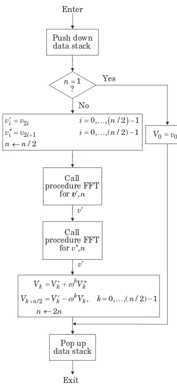
4.8 A recursive radix-two fast Fourier transform 139
5
Fast algorithms for short convolutions
1455.1 Cyclic convolution and linear convolution 145
5.2 The Cook–Toom algorithm 148
5.3 Winograd short convolution algorithms 155
5.4 Design of short linear convolution algorithms 164
5.5 Polynomial products modulo a polynomial 168
5.6 Design of short cyclic convolution algorithms 171
5.7 Convolution in general fields and rings 176
5.8 Complexity of convolution algorithms 178
6
Architecture of filters and transforms
1946.1 Convolution by sections 194
6.2 Algorithms for short filter sections 199
6.3 Iterated filter sections 202
6.4 Symmetric and skew-symmetric filters 207
6.5 Decimating and interpolating filters 213
6.6 Construction of transform computers 216
6.7 Limited-range Fourier transforms 221
ix Contents
7
Fast algorithms for solving Toeplitz systems
2317.1 The Levinson and Durbin algorithms 231
7.2 The Trench algorithm 239
7.3 Methods based on the euclidean algorithm 245
7.4 The Berlekamp–Massey algorithm 249
7.5 An accelerated Berlekamp–Massey algorithm 255
8
Fast algorithms for trellis search
2628.1 Trellis and tree searching 262
8.2 The Viterbi algorithm 267
8.3 Sequential algorithms 270
8.4 The Fano algorithm 274
8.5 The stack algorithm 278
8.6 The Bahl algorithm 280
9
Numbers and fields
2869.1 Elementary number theory 286
9.2 Fields based on the integer ring 293
9.3 Fields based on polynomial rings 296
9.4 Minimal polynomials and conjugates 299
9.5 Cyclotomic polynomials 300
9.6 Primitive elements 304
9.7 Algebraic integers 306
10
Computation in finite fields and rings
31110.1 Convolution in surrogate fields 311
10.2 Fermat number transforms 314
10.3 Mersenne number transforms 317
10.4 Arithmetic in a modular integer ring 320
10.5 Convolution algorithms in finite fields 324
10.6 Fourier transform algorithms in finite fields 328
10.8 Integer ring transforms 336
10.9 Chevillat number transforms 339
10.10 The Preparata–Sarwate algorithm 339
11
Fast algorithms and multidimensional convolutions
34511.1 Nested convolution algorithms 345
11.2 The Agarwal–Cooley convolution algorithm 350
11.3 Splitting algorithms 357
11.4 Iterated algorithms 362
11.5 Polynomial representation of extension fields 368
11.6 Convolution with polynomial transforms 371
11.7 The Nussbaumer polynomial transforms 372
11.8 Fast convolution of polynomials 376
12
Fast algorithms and multidimensional transforms
38412.1 Small-radix Cooley–Tukey algorithms 384
12.2 The two-dimensional discrete cosine transform 389
12.3 Nested transform algorithms 391
12.4 The Winograd large fast Fourier transform 395
12.5 The Johnson–Burrus fast Fourier transform 399
12.6 Splitting algorithms 403
12.7 An improved Winograd fast Fourier transform 410
12.8 The Nussbaumer–Quandalle permutation algorithm 411
A
A collection of cyclic convolution algorithms
427B
A collection of Winograd small FFT algorithms
435Bibliography 442
Preface
A quarter of a century has passed since the previous version1of this book was published, and signal processing continues to be a very important part of electrical engineering. It forms an essential part of systems for telecommunications, radar and sonar, image formation systems such as medical imaging, and other large computational problems, such as in electromagnetics or fluid dynamics, geophysical exploration, and so on. Fast computational algorithms are necessary in large problems of signal processing, and the study of such algorithms is the subject of this book. Over those several decades, however, the nature of the need for fast algorithms has shifted both to much larger systems on the one hand and to embedded power-limited applications on the other.
Because many processors and many problems are much larger now than they were when the original version of this book was written, and the relative cost of addition and multiplication now may appear to be less dramatic, some of the topics of twenty years ago may be seen by some to be of less importance today. I take exactly the opposite point of view for several reasons. Very large three-dimensional or four-dimensional problems now under consideration require massive amounts of computation and this computation can be reduced by orders of magnitude in many cases by the choice of algorithm. Indeed, these very large problems can be especially suitable for the benefits of fast algorithms. At the same time, smaller signal processing problems now appear frequently in handheld or remote applications where power may be scarce or nonrenewable. The designer’s care in treating an embedded application, such as a digital television, can repay itself many times by significantly reducing the power expenditure. Moreover, the unfamiliar algorithms of this book now can often be handled automatically by computerized design tools, and in embedded applications where power dissipation must be minimized, a search for the algorithm with the fewest operations may be essential.
Because the book has changed in its details and the title has been slightly modernized, it is more than a second edition, although most of the topics of the original book have been retained in nearly the same form, but usually with the presentation rewritten. Possibly, in time, some of these topics will re-emerge in a new form, but that time
is not now. A newly written book might look different in its choice of topics and its balance between topics than does this one. To accommodate this consideration here, the chapters have been rearranged and revised, even those whose content has not changed substantially. Some new sections have been added, and all of the book has been polished, revised, and re-edited. Most of the touch and feel of the original book is still evident in this new version.
The heart of the book is in the Fourier transform algorithms of Chapters3and12
and the convolution algorithms of Chapters5and11. Chapters12and11are the multi-dimensional continuations of Chapters3and4, respectively, and can be partially read immediately thereafter if desired. The study of one-dimensional convolution algorithms and Fourier transform algorithms is only completed in the context of the multidimen-sional problems. Chapters 2 and 9 are mathematical interludes; some readers may prefer to treat them as appendices, consulting them only as needed. The remainder, Chapters4,7, and8, are in large part independent of the rest of the book. Each can be read independently with little difficulty.
Acknowledgments
My major debt in writing this book is to Shmuel Winograd. Without his many con-tributions to the subject, the book would be shapeless and much shorter. He was also generous with his time in clarifying many points to me, and in reviewing early drafts of the original book. The papers of Winograd and also the book of Nussbaumer were a source for much of the material discussed in this book.
The original version of this book could not have reached maturity without being tested, critiqued, and rewritten repeatedly. I remain indebted to Professor B. W. Dickinson, Professor Toby Berger, Professor C. S. Burrus, Professor J. Gibson, Pro-fessor J. G. Proakis, ProPro-fessor T. W. Parks, Dr B. Rice, ProPro-fessor Y. Sugiyama, Dr W. Vanderkulk, and Professor G. Verghese for their gracious criticisms of the original 1985 manuscript. That book could not have been written without the support that was given by the International Business Machines Corporation. I am deeply grate-ful to IBM for this support and also to Cornell University for giving me the opportunity to teach several times from the preliminary manuscript of the earlier book. The revised book was written in the wonderful collaborative environment of the Department of Electrical and Computer Engineering and the Coordinated Science Laboratory of the University of Illinois. The quality of the book has much to with the composition skills of Mrs Francie Bridges and the editing skills of Mrs Helen Metzinger. And, as always, Barbara made it possible.
1
Introduction
Algorithms for computation are found everywhere, and efficient versions of these algorithms are highly valued by those who use them. We are mainly concerned with certain types of computation, primarily those related to signal processing, including the computations found in digital filters, discrete Fourier transforms, correlations, and spectral analysis. Our purpose is to present the advanced techniques for fast digital implementation of these computations. We are not concerned with the function of a digital filter or with how it should be designed to perform a certain task; our concern is only with the computational organization of its implementation. Nor are we concerned with why one should want to compute, for example, a discrete Fourier transform; our concern is only with how it can be computed efficiently. Surprisingly, there is an extensive body of theory dealing with this specialized topic – the topic of fast algorithms.
1.1
Introduction to fast algorithms
An algorithm, like most other engineering devices, can be described either by an input/output relationship or by a detailed explanation of its internal construction. When one applies the techniques of signal processing to a new problem one is concerned only with the input/output aspects of the algorithm. Given a signal, or a data record of some kind, one is concerned with what should be done to this data, that is, with what the output of the algorithm should be when such and such a data record is the input. Perhaps the output is a filtered version of the input, or the output is the Fourier transform of the input. The relationship between the input and the output of a computational task can be expressed mathematically without prescribing in detail all of the steps by which the calculation is to be performed.
Devising such an algorithm for an information processing problem, from this input/output point of view, may be a formidable and sophisticated task, but this is not our concern in this book. We will assume that we are given a specification of a relationship between input and output, described in terms of filters, Fourier transforms, interpolations, decimations, correlations, modulations, histograms, matrix operations,
and so forth. All of these can be expressed with mathematical formulas and so can be computed just as written. This will be referred to as the obvious implementation.
One may be content with the obvious implementation, and it might not be apparent that the obvious implementation need not be the most efficient. But once people began to compute such things, other people began to look for more efficient ways to compute them. This is the story we aim to tell, the story of fast algorithms for signal processing. By a fast algorithm, we mean a detailed description of a computational procedure that is not the obvious way to compute the required output from the input. A fast algorithm usually gives up a conceptually clear computation in favor of one that is computationally efficient.
Suppose we need to compute a numberA, given by
A=ac+ad+bc+bd.
As written, this requires four multiplications and three additions to compute. If we need to computeAmany times with different sets of data, we will quickly notice that
A=(a+b)(c+d)
is an equivalent form that requires only one multiplication and two additions, and so it is to be preferred. This simple example is quite obvious, but really illustrates most of what we shall talk about. Everything we do can be thought of in terms of the clever insertion of parentheses in a computational problem. But in a big problem, the fast algorithms cannot be found by inspection. It will require a considerable amount of theory to find them.
A nontrivial yet simple example of a fast algorithm is an algorithm for complex multiplication. The complex product1
(e+jf)=(a+jb)·(c+jd)
can be defined in terms of real multiplications and real additions as
e=ac−bd f =ad+bc.
We see that these formulas require four real multiplications and two real additions. A more efficient “algorithm” is
e=(a−b)d+a(c−d)
f =(a−b)d+b(c+d)
whenever multiplication is harder than addition. This form requires three real multi-plications and five real additions. If c and d are constants for a series of complex
3 1.1 Introduction to fast algorithms
multiplications, then the termsc+dandc−dare constants also and can be computed off-line. It then requires three real multiplications and three real additions to do one complex multiplication.
We have traded one multiplication for an addition. This can be a worthwhile saving, but only if the signal processor is designed to take advantage of it. Most signal pro-cessors, however, have been designed with a prejudice for a complex multiplication that uses four multiplications. Then the advantage of the improved algorithm has no value. The storage and movement of data between additions and multiplications are also important considerations in determining the speed of a computation and of some importance in determining power dissipation.
We can dwell further on this example as a foretaste of things to come. The complex multiplication above can be rewritten as a matrix product
e f = c −d
d c
a b
,
where the vector
a b
represents the complex numbera+jb, the matrix
c −d
d c
represents the complex number c+jd, and the vector
e f
represents the complex
number e+jf. The matrix–vector product is an unconventional way to represent complex multiplication. The alternative computational algorithm can be written in matrix form as
e f =
1 0 1
0 1 1
(c−d) 0 0 0 (c+d) 0
0 0 d
1 0 0 1
1 −1
a b .
The algorithm, then, can be thought of as nothing more than the unusual matrix factorization:
c −d
d c
=
1 0 1
0 1 1
(c−d) 0 0 0 (c+d) 0
0 0 d
1 0 0 1
1 −1
.
We can abbreviate the algorithm as
e f
= B D A
a b
,
We shall find that many fast computational procedures for convolution and for the discrete Fourier transform can be put into this factored form of a diagonal matrix in the center, and on each side of which is a matrix whose elements are 1, 0, and−1. Multiplication by a matrix whose elements are 0 and±1 requires only additions and subtractions. Fast algorithms in this form will have the structure of a batch of additions, followed by a batch of multiplications, followed by another batch of additions.
The final example of this introductory section is a fast algorithm for multiplying two arbitrary matrices. Let
C = AB,
whereAandBare anyℓbyn, andnbym, matrices, respectively. The standard method for computing the matrixCis
cij = n
k=1
aikbkj
i =1, . . . , ℓ j =1, . . . , m,
which, as it is written, requiresmℓnmultiplications and (n−1)ℓmadditions. We shall give an algorithm that reduces the number of multiplications by almost a factor of two but increases the number of additions. The total number of operations increases slightly.
We use the identity
a1b1+a2b2 =(a1+b2)(a2+b1)−a1a2−b1b2
on the elements of A and B. Suppose thatnis even (otherwise append a column of zeros to Aand a row of zeros to B, which does not change the productC). Apply the above identity to pairs of columns of Aand pairs of rows of Bto write
cij = n/2
i=1
(ai,2k−1b2k−1,j +ai,2kb2k,j)
=
n/2
k=1
(ai,2k−1+b2k,j)(ai,2k+b2k−1,j)− n/2
k=1
ai,2k−1ai,2k− n/2
k=1
b2k−1,jb2k,j
fori=1, . . . , ℓandj =1, . . . , m.
This results in computational savings because the second term depends only on
i and need not be recomputed for each j, and the third term depends only on j
and need not be recomputed for each i. The total number of multiplications used to compute matrix C is 12nℓm+12n(ℓ+m), and the total number of additions is
3
2nℓm+ℓm+
1 2n−1
(ℓ+m). For large matrices the number of multiplications is about half the direct method.
5 1.1 Introduction to fast algorithms
Algorithm Multiplications/pixel* Additions/pixel
Direct computation of discrete Fourier transform
1000 x 1000
8000 4000
Basic Cooley–Tukey FFT 1024 x 1024
40 60
Hybrid Cooley– Tukey/Winograd FFT
1000 x 1000
40 72.8
Winograd FFT 1008 x 1008
6.2 91.6
Nussbaumer–Quandalle FFT 1008 x 1008
4.1 79
*1 pixel – 1 output grid point
Figure 1.1 Relative performance of some two-dimensional Fourier transform algorithms
however, one can obtain computational accuracy that is nearly the same as the direct method. Consideration of computational noise is always a practical factor in judging a fast algorithm, although we shall usually ignore it. Sometimes when the number of operations is reduced, the computational noise is reduced because fewer computations mean that there are fewer sources of noise. In other algorithms, though there are fewer sources of computational noise, the result of the computation may be more sensitive to one or more of them, and so the computational noise in the result may be increased. Most of this book will be spent studying only a few problems: the problems of linear convolution, cyclic convolution, multidimensional linear convolution, multi-dimensional cyclic convolution, the discrete Fourier transform, the multimulti-dimensional discrete Fourier transforms, the solution of Toeplitz systems, and finding paths in a trellis. Some of the techniques we shall study deserve to be more widely used – multidimensional Fourier transform algorithms can be especially good if one takes the pains to understand the most efficient ones. For example, Figure 1.1 compares some methods of computing a two-dimensional Fourier transform. The improvements in performance come more slowly toward the end of the list. It may not seem very important to reduce the number of multiplications per output cell from six to four after the reduction has already gone from forty to six, but this can be a shortsighted view. It is an additional savings and may be well worth the design time in a large application. In power-limited applications, a potential of a significant reduction in power may itself justify the effort.
that one should use only a power of two blocklength; good algorithms are available for many values of the blocklength.
1.2
Applications of fast algorithms
Very large scale integrated circuits, or chips, are now widely available. A modern chip can easily contain many millions of logic gates and memory cells, and it is not surprising that the theory of algorithms is looked to as a way to efficiently organize these gates on special-purpose chips. Sometimes a considerable performance improvement, either in speed or in power dissipation, can be realized by the choice of algorithm. Of course, a performance improvement in speed can also be realized by increasing the size or the speed of the chip. These latter approaches are more widely understood and easier to design, but they are not the only way to reduce power or chip size.
For example, suppose one devises an algorithm for a Fourier transform that has only one-fifth of the computation of another Fourier transform algorithm. By using the new algorithm, one might realize a performance improvement that can be as real as if one increased the speed or the size of the chip by a factor of five. To realize this improvement, however, the chip designer must reflect the architecture of the algorithm in the architecture of the chip. A naive design can dissipate the advantages by increasing the complexity of indexing, for example, or of data flow between computational steps. An understanding of the fast algorithms described in this book will be required to obtain the best system designs in the era of very large-scale integrated circuits.
At first glance, it might appear that the two kinds of development – fast circuits and fast algorithms – are in competition. If one can build the chip big enough or fast enough, then it seemingly does not matter if one uses inefficient algorithms. No doubt this view is sound in some cases, but in other cases one can also make exactly the opposite argument. Large digital signal processors often create a need for fast algorithms. This is because one begins to deal with signal-processing problems that are much larger than before. Whether competing algorithms for some problem of interest have running times proportional ton2orn3may be of minor importance whennequals three or four; but whennequals 1000, it becomes critical.
7 1.2 Applications of fast algorithms
We usually measure the performance of an algorithm by the number of multipli-cations and additions it uses. These performance measures are about as deep as one can go at the level of the computational algorithm. At a lower level, we would want to know the area of the chip or the number of gates on it and the time required to complete a computation. Often one judges a circuit by the area–time product. We will not give performance measures at this level because this is beyond the province of the algorithm designer, and entering the province of the chip architecture.
The significance of the topics in this book cannot be appreciated without under-standing the massive needs of some processing applications of the near future and the power limitations of other embedded applications now in widespread use. At the present time, applications are easy to foresee that require orders of magnitude more signal processing than current technology can satisfy.
Sonar systems have now become almost completely digital. Though they process only a few kilohertz of signal bandwidth, these systems can use hundreds of millions of multiplications per second and beyond, and even more additions. Extensive racks of digital equipment may be needed for such systems, and yet reasons for even more processing in sonar systems are routinely conceived.
Radar systems also have become digital, but many of the front-end functions are still done by conventional microwave or analog circuitry. In principle, radar and sonar are quite similar, but radar has more than one thousand times as much band-width. Thus, one can see the enormous potential for digital signal processing in radar systems.
Seismic processing provides the principal method for exploration deep below the Earth’s surface. This is an important method of searching for petroleum reserves. Many computers are already busy processing the large stacks of seismic data, but there is no end to the seismic computations remaining to be done.
Computerized tomography is now widely used to synthetically form images of internal organs of the human body by using X-ray data from multiple projections. Improved algorithms are under study that will reduce considerably the X-ray dosage, or provide motion or function to the imagery, but the signal-processing requirements will be very demanding. Other forms of medical imaging continue to advance, such as those using ultrasonic data, nuclear magnetic resonance data, or particle decay data. These also use massive amounts of digital signal processing.
manufactured articles, such as castings, is possible by means of computer-generated internal images based on the response to induced acoustic vibrations.
Other applications for the fast algorithms of signal processing could be given, but these should suffice to prove the point that a need exists and continues to grow for fast signal-processing algorithms.
All of these applications are characterized by computations that are massive but are fairly straightforward and have an orderly structure. In addition, in such applications, once a hardware module or a software subroutine is designed to do a certain task, it is permanently dedicated to this task. One is willing to make a substantial design effort because the design cost is not what matters; the operational performance, both speed and power dissipation, is far more important.
At the same time, there are embedded applications for which power reduction is of critical importance. Wireless handheld and desktop devices and untethered remote sensors must operate from batteries or locally generated power. Chips for these devices may be produced in the millions. Nonrecurring design time to reduce the computations needed by the required algorithm is one way to reduce the power requirements.
1.3
Number systems for computation
Throughout the book, when we speak of the complexity of an algorithm, we will cite the number of multiplications and additions, as if multiplications and additions were fundamental units for measuring complexity. Sometimes one may want to go a little deeper than this and look at how the multiplier is built so that the number of bit operations can be counted. The structure of a multiplier or adder critically depends on how the data is represented. Though we will not study such issues of number representation, a few words are warranted here in the introduction.
To take an extreme example, if a computation involves mostly multiplication, the complexity may be less if the data is provided in the form of logarithms. The additions will now be more complicated; but if there are not too many additions, a savings will result. This is rarely the case, so we will generally assume that the input data is given in its natural form either as real numbers, as complex numbers, or as integers.
9 1.4 Digital signal processing
and the recurring manufacturing costs that matter. Money spent on features to ease the designer’s work cannot be spent to increase performance.
A nonnegative integer j smaller than qm has an m-symbol fixed-point radix-q representation, given by
j =j0+j1q+j2q2+ · · · +jm−1qm−1, 0≤ji < q.
The integerj is represented by them-tuple of coefficients (j0, j1, . . . , jm−1). Several methods are used to handle the sign of a fixed-point number. These are sign-and-magnitude numbers,q-complement numbers, and (q−1)-complement numbers. The same techniques can be used for numbers expressed in any base. In a binary notation,q
equals two, and the complement representations are called two’s-complement numbers and one’s-complement numbers.
The sign-and-magnitude convention is easiest to understand. The magnitude of the number is augmented by a special digit called the sign digit; it is zero – indicating a plus sign – for positive numbers and it is one – indicating a minus sign – for negative numbers. The sign digit is treated differently from the magnitude digits during addition and multiplication, in the customary way. The complement notations are a little harder to understand, but often are preferred because the hardware is simpler; an adder can simply add two numbers, treating the sign digit the same as the magnitude digits. The sign-and-magnitude convention and the (q−1)-complement convention each leads to the existence of both a positive and a negative zero. These are equal in meaning, but have separate representations. The two’s-complement convention in binary arithmetic and the ten’s-complement convention in decimal arithmetic have only a single representation for zero.
The (q−1)-complement notation represents the negative of a number by replacing digit j, including the sign digit, by q−1−j. For example, in nine’s-complement notation, the negative of the decimal number+62, which is stored as 062, is 937; and the negative of the one’s-complement binary number+011, which is stored as 0011, is 1100. The (q−1)-complement representation has the feature that one can multiply any number by minus one simply by taking the (q−1)-complement of each digit.
The q-complement notation represents the negative of a number by adding one to the (q−1)-complement notation. The negative of zero is zero. In this convention, the negative of the decimal number+62, which is stored as 062, is 938; and the negative of the binary number+011, which is stored as 0011, is 1101.
1.4
Digital signal processing
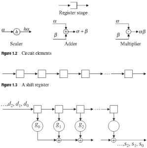
Figure 1.2 Circuit elements
Figure 1.3 A shift register
g
0g
1g
2…,s
2, s
1, s
0,
d
2,
d
1,
d
0Figure 1.4 A finite-impulse-response filter
processing. The numbers in the sequence are usually either real numbers or complex numbers, but other kinds of number sometimes occur. A digital filter is a device that produces a new sequence of numbers, called the output sequence, from the given sequence, now called theinput sequence. Filters in common use can be constructed out of those circuit elements, illustrated in Figure1.2, calledshift-register stages,adders, scalers, andmultipliers. A shift-register stage holds a single number, which it displays on its output line. At discrete time instants calledclock times, the shift-register stage replaces its content with the number appearing on the input line, discarding its previous content. A shift register, illustrated in Figure1.3, is a number of shift-register stages connected in a chain.
11 1.4 Digital signal processing
1 L
i j i j i
p
h p
a
1
j
Figure 1.5 An autoregressive filter
Linear convolution is perhaps the most common computational problem found in signal processing, and we shall spend a great deal of time studying how to implement it efficiently. We shall spend even more time studying ways to compute a cyclic convolution. This may seem a little strange because a cyclic convolution does not often arise naturally in applications. We study it because there are so many good ways to compute a cyclic convolution. Therefore we will develop fast methods of computing long linear convolutions by patching together many cyclic convolutions.
Given the two sequences called thedata sequence
d= {di |i =0, . . . , N−1} and thefilter sequence
g= {gi |i=0, . . . , L−1},
whereNis the data blocklength andLis the filter blocklength, the linear convolution is a new sequence called thesignal sequenceor theoutput sequence
s= {si |i=0, . . . , L+N−2}, given by the equation
si = N−1
k=0
gi−kdk, i=0, . . . , L+N−2,
andL+N−1 is the output blocklength. The convolution is written with the under-standing thatgi−k =0 ifi−k is less than zero. Because each component ofd mul-tiplies, in turn, each component of g, there are N L multiplications in the obvious implementation of the convolution.
A concept closely related to the convolution is the correlation, given by
ri = N−1
k=0
gi+kdk, i=0, . . . , L+N−2,
wheregi+k =0 fori+k≥L. The correlation can be computed as a convolution simply by reading one of the two sequences backwards. All of the methods for computing a linear convolution are easily changed into methods for computing the correlation.
We can also express the convolution in the notation of polynomials. Let
d(x)= N−1
i=0
dixi,
g(x)= L−1
i=0
gixi.
Then
s(x)=g(x)d(x),
where
s(x)= L+N−2
i=0
sixi.
This can be seen by examining the coefficients of the productg(x)d(x). Of course, we can also write
s(x)=d(x)g(x),
which makes it clear thatdandgplay symmetric roles in the convolution. Therefore we can also write the linear convolution in the equivalent form
si = L−1
k=0
gkdi−k.
Another form of convolution is thecyclic convolution, which is closely related to the linear convolution. Given the two sequencesdi for i=0, . . . , n−1 and gi for i=0, . . . , n−1, each of blocklengthn, a new sequences′
i for i=0, . . . , n−1 of blocklengthnnow is given by the cyclic convolution
si′= n−1
k=0
g((i−k))dk, i=0, . . . , n−1,
where the double parentheses denote modulo n arithmetic on the indices (see Section2.6). That is,
13 1.4 Digital signal processing
and
0≤((i−k))< n.
Notice that in the cyclic convolution, for everyi, everydkfinds itself multiplied by a meaningful value ofg((i−k)). This is different from the linear convolution where, for somei,dkwill be multiplied by agi−k whose index is outside the range of definition ofg, and so is zero.
We can relate the cyclic convolution outputs to the linear convolution as follows. By the definition of the cyclic convolution
si′ = n−1
k=0
g((i−k))dk, i=0, . . . , n=1.
We can recognize two kinds of term in the sum: those withi−k≥0 and those with
i−k <0. Those occur whenk≤iandk > i, respectively. Hence
si′ = i
k=0
gi−kdk+ n−1
k=i+1
gn+i−kdk.
But now, in the first sum,gi−k =0 ifk > i; and in the second sum,gn+i−k=0 ifk < i. Hence we can change the limits of the summations as follows:
si′ = n−1
k=0
gi−kdk+ n−1
k=0
gn+i−kdk, i=0, . . . , n−1
=si +sn+i, i=0, . . . , n−1,
which relates the cyclic convolution outputs on the left to the linear convolution outputs on the right. We say that coefficients of swith index larger than n−1 are “folded” back into terms with indices smaller thann.
The linear convolution can be computed as a cyclic convolution if the second term above equals zero. This is so ifgn+i−kdkequals zero for alliandk. To ensure this, one can choosen, the blocklength of the cyclic convolution, so thatnis larger thanL+ N−2 (appending zeros toganddso their blocklength isn). Then one can compute the linear convolution by using an algorithm for computing a cyclic convolution and still get the right answer.
The cyclic convolution can also be expressed as a polynomial product. Let
d(x)= n−1
i=0
dixi,
g(x)= n−1
i=0
Repeat input
1, , 1, 0, 1, , 1, 0
n n
d d d d d d
0
g g1 gn1
0 1 1 Select middle
cyclic convolution
, , , n
n points for
xxxx s s xxx s
Figure 1.6 Using a FIR filter to form cyclic convolutions
Whereas the linear convolution is represented by
s(x)=g(x)d(x),
the cyclic convolution is computed by folding back the high-order coefficients ofs(x) by writing
s′(x)=g(x)d(x) (modxn−1).
By the equality modulo xn−1, we mean that s′(x) is the remainder when s(x) is
divided byxn−1. To reduceg(x)d(x) moduloxn−1, it suffices to replacexnby one, or to replace xn+i byxi wherever a term xn+i withi positive appears. This has the effect of forming the coefficients
si′=si+sn+i, i =0, . . . , n−1
and so gives the coefficients of the cyclic convolution. From the two forms
s′(x)=d(x)g(x) (modxn−1) =g(x)d(x) (modxn−1),
it is clear that the roles of d and g are also symmetric in the cyclic convolution. Therefore we have the two expressions for the cyclic convolution
si′= n−1
k=0
g((i−k))dk, i=0, . . . , n−1
=
n−1
k=0
d((i−k))gk, i=0, . . . , n−1.
15 1.4 Digital signal processing
those 3n−1 outputs is a consecutive sequence ofnoutputs that is equal to the cyclic convolution.
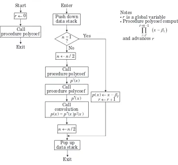
A more important technique is to use a cyclic convolution to compute a long linear convolution. Fast algorithms for long linear convolutions break the input datastream into short sections of perhaps a few hundred samples. One section at a time is processed – often as a cyclic convolution – to produce a section of the output datastream. Techniques for doing this are calledoverlaptechniques, referring to the fact that nonoverlapping sections of the input datastream cause overlapping sections of the output datastream, while nonoverlapping sections of the output datastream are caused by overlapping sections of the input datastream. Overlap techniques are studied in detail in Chapter5. The operation of an autoregressive filter, as was shown in Figure 1.5, also can be described in terms of polynomial arithmetic. Whereas the finite-impulse-response filter computes a polynomial product, an autoregressive filter computes a polynomial division. Specifically, when a finite sequence is filtered by an autoregressive filter (with zero initial conditions), the output sequence corresponds to the quotient polynomial under polynomial division by the polynomial whose coefficients are the tap weights, and at the instant when the input terminates, the register contains the corresponding remainder polynomial. In particular, recall that the output pj of the autoregressive filter, by appropriate choice of the signs of the tap weights,hi, is given by
pj = − L j=1
hipj−i+aj,
whereaj is thejth input symbol andhi is the weight of theith tap of the filter. Define the polynomials
a(x)= n j=0
ajxj
and
h(x)= L j=0
hjxj,
and write
a(x)=Q(x)h(x)+r(x),
whereQ(x) andr(x) are the quotient polynomial and the remainder polynomial under division of polynomials. We conclude that the filter output pj is equal to the jth coefficient of the quotient polynomial, sop(x)=Q(x). The coefficients of the remain-der polynomial r(x) will be left in the stages of the autoregressive filter after the n
coefficientsajare shifted in.
v=[vi |i =0, . . . , n−1] be a vector of complex numbers or a vector of real num-bers. The Fourier transform ofvis another vectorV of lengthnof complex numbers, given by
Vk = n−1
i=0
ωikvi, k =0, . . . , n−1,
whereω=e−j2π/nand j=√−1.
Sometimes we write this computation as a matrix–vector product
V = Tv.
When written out, this becomes
V0 V1 V2 .. .
Vn−1
=
1 1 1 · · · 1
1 ω ω2 · · · ωn−1 1 ω2 ω4 · · · ω2(n−1)
..
. ... ...
1 ωn−1 ω2(n−1) · · · ω v0 v1 v2 .. .
vn−1
.
If V is the Fourier transform ofv, thenvcan be recovered fromV by the inverse Fourier transform, which is given by
vi = 1
n n−1
k=0
ω−ikVk.
The proof is as follows:
n−1
k=0
ω−ikVk = n−1
k=0
ω−ik n−1
ℓ=0
ωℓkvℓ
=
n−1
ℓ=0
vℓ n−1
k=0
ωk(ℓ−i)
.
But the summation onkis clearly equal tonifℓis equal toi, while ifℓis not equal to
ithe summation becomes n−1
k=0
(ω(ℓ−i))k = 1−ω (ℓ−i)n 1−ω(ℓ−i).
The right side equals zero becauseωn=1 and the denominator is not zero. Hence n−1
k=0
ω−ikVk = n−1
ℓ=0
vℓ(nδiℓ) = nvi,
17 1.5 History of fast signal-processing algorithms
There is an important link between the Fourier transform and the cyclic convolution. This link is known as the convolution theoremand goes as follows. The vector e is given by the cyclic convolution of the vectors f andg:
ei = n−1
ℓ=0
f((i−ℓ))gℓ, i=0, . . . , n−1,
if and only if the Fourier transforms satisfy
Ek =FkGk, k =0, . . . , n−1. This holds because
ei = n−1
ℓ=0
f((i−ℓ))
1
n n−1
k=0
ω−kℓGk
= 1
n n−1
k=0
ω−ikGk n−1
ℓ=0
ω(i−ℓ)kf((i−ℓ))
= 1
n n−1
k=0
ω−ikGkFk.
Becauseeis the inverse Fourier transform ofE, we conclude thatEk=GkFk. There are also two-dimensional Fourier transforms, which are useful for processing two-dimensional arrays of data, and multidimensional Fourier transforms, which are useful for processing multidimensional arrays of data. The two-dimensional Fourier transform on ann′byn′′array is
Vk′k′′ =
n′−1
i′=0
n′′−1
i′′=0
ωi′k′µi′′k′′vi′i′′,
k′ = 0, . . . , n′−1,
k′′ = 0, . . . , n′′−1,
where ω=e−j2π/n′
andµ=e−j2π/n′′
. Chapter12is devoted to the two-dimensional Fourier transforms.
1.5
History of fast signal-processing algorithms
at the time it was published. Later, a more efficient though more complicated algo-rithm was published by Winograd (1976, 1978), who also provided a much deeper understanding of what it means to compute the Fourier transform.
The radix-two Cooley–Tukey FFT is especially elegant and efficient, and so is very popular. This has led some to the belief that the discrete Fourier transform is practical only if the blocklength is a power of two. This belief tends to result in the FFT algorithm dictating the design parameters of an application rather than the application dictating the choice of FFT algorithm. In fact, there are good FFT algorithms for just about any blocklength.
The Cooley–Tukey FFT, in various guises, has appeared independently in other contexts. Essentially the same idea is known as the Butler matrix (1961) when it is used as a method of wiring a multibeam phased-array radar antenna.
Fast convolution algorithms of small blocklength were first constructed by Agar-wal and Cooley (1977) using clever insights but without a general technique. Wino-grad (1978) gave a general method of construction and also proved important theorems concerning the nonexistence of better convolution algorithms in the real field or the complex field. Agarwal and Cooley (1977) also found a method to break long con-volutions into short concon-volutions using the Chinese remainder theorem. Their method works well when combined with the Winograd algorithm for short convolutions.
The earliest idea of modern signal processing that we label as a fast algorithm came much earlier than the FFT. In 1947 the Levinson algorithm was published as an efficient method of solving certain Toeplitz systems of equations. Despite its great importance in the processing of seismic signals, the literature of the Levinson algorithm remained disjoint from the literature of the FFT for many years. Generally, the early literature does not distinguish carefully between the Levinson algorithm as a computational pro-cedure and the filtering problem to which the algorithm might be applied. Similarly, the literature does not always distinguish carefully between the FFT as a computa-tional procedure and the discrete Fourier transform to which the FFT is applied, nor between the Viterbi algorithm as a computational procedure and the minimum-distance pathfinding problem to which the Viterbi algorithm is applied.
Problems for Chapter 1
1.1 Construct an algorithm for the two-point real cyclic convolution
(s1x+s0)=(g1x+g0)(d1x+d0) (modx2−1)
that uses two multiplications and four additions. Computations involving only
19 Problems
1.2 Using the result of Problem 1.1, construct an algorithm for the two-point complex cyclic convolution that uses only six real multiplications.
1.3 Construct an algorithm for the three-point Fourier transform
Vk =
2
i=0
ωikvi, k=0,1,2
that uses two real multiplications.
1.4 Prove that there does not exist an algorithm for multiplying two complex num-bers that uses only two real multiplications. (A throughful “proof” will struggle with the meaning of the term “multiplication.”)
1.5 a Suppose you are given a device that computes the linear convolution of two fifty-point sequences. Describe how to use it to compute the cyclic convolution of two fifty-point sequences.
b Suppose you are given a device that computes the cyclic convolution of two fifty-point sequences. Describe how to use it to compute the linear convolution of two fifty-point sequences.
1.6 Prove that one can compute a correlation as a convolution by writing one of the sequences backwards, possibly padding a sequence with a string of zeros. 1.7 Show that any algorithm for computingx31that uses only additions, subtractions,
and multiplications must use at least seven multiplications, but that if division is allowed, then an algorithm exists that uses a total of six multiplications and divisions.
1.8 Another algorithm for complex multiplication is given by
e=ac−bd,
f =(a+b)(c+d)−ac−bd.
Express this algorithm in a matrix form similar to that given in the text. What advantages or disadvantages are there in this algorithm?
1.9 Prove the “translation property” of the Fourier transform. If{vj} ↔ {Vk} is a Fourier transform pair, then the following are Fourier transform pairs:
{ωivi} ↔ {V((k+1))}, {v((i−1))} ↔ {ωkVk}.
1.10 Prove that the “cyclic correlation” in the real field satisfies the Fourier transform relationship
GkDk∗↔ n−1
k=0
g((i+k))dk.
Notes for Chapter 1
A good history of the origins of the fast Fourier transform algorithms is given in a paper by Cooley, Lewis, and Welch (1967). The basic theory of digital signal processing can be found in many books, including the books by Oppenheim and Shafer (1975), Rabiner and Gold (1975), and Proakis and Manolakis (2006).
2
Introduction to abstract algebra
Good algorithms are elegant algebraic identities. To construct these algorithms, we must be familiar with the powerful structures of number theory and of modern algebra. The structures of the set of integers, of polynomial rings, and of Galois fields will play an important role in the design of signal-processing algorithms. This chapter will introduce those mathematical topics of algebra that will be important for later developments but that are not always known to students of signal processing. We will first study the mathematical structures of groups, rings, and fields. We shall see that a discrete Fourier transform can be defined in many fields, though it is most familiar in the complex field. Next, we will discuss the familiar topics of matrix algebra and vector spaces. We shall see that these can be defined satisfactorily in any field. Finally, we will study the integer ring and polynomial rings, with particular attention to the euclidean algorithm and the Chinese remainder theorem in each ring.
2.1
Groups
A group is a mathematical abstraction of an algebraic structure that appears frequently in many concrete forms. The abstract idea is introduced because it is easier to study all mathematical systems with a common structure at once, rather than to study them one by one.
Definition 2.1.1 A groupGis a set together with an operation(denoted by∗)satisfying four properties.
1 (Closure)For everyaandbin the set,c=a∗bis in the set. 2 (Associativity)For everya,b, andcin the set,
a∗(b∗c)=(a∗b)∗c.
3 (Identity)There is an elementecalled the identity element that satisfies
a∗e=e∗a=a
for everyain the setG.
1 2 3 4
1 2 3 4
1 1 2 3 4
2 2 3 4 1
3 3 4 1 2
4 4 1 2 3
e g g g g
e e g g g g
g g g g e
g g g e g
g g e g g
g e g g g
0 1 2 3 4 0 0 1 2 3 4 1 1 2 3 4 0 2 2 3 4 0 1 3 3 4 0 1 2 4 4 0 1 2 3
g g g g
Figure 2.1 Example of a finite group
4 (Inverses)Ifais in the set, then there is some elementbin the set called an inverse of a such that
a∗b=b∗a=e.
A group that has a finite number of elements is called afinite group. The number of elements in a finite groupGis called theorderofG. An example of a finite group is shown in Figure2.1. The same group is shown twice, but represented by two different notations. Whenever two groups have the same structure but a different representation, they are said to beisomorphic.1
Some groups satisfy the property that for allaandbin the group
a∗b=b∗a.
This is called the commutative property. Groups with this additional property are called commutative groups or abelian groups. We shall usually deal with abelian groups.
In an abelian group, the symbol for the group operation is commonly written+and is called addition (even though it might not be the usual arithmetic addition). Then the identity elemente is called “zero” and is written 0, and the inverse element ofa is written−aso that
a+(−a)=(−a)+a=0.
Sometimes the symbol for the group operation is written∗and is called multiplication (even though it might not be the usual arithmetic multiplication). In this case, the identity element e is called “one” and is written 1, and the inverse element ofa is writtena−1so that
a∗a−1=a−1∗a=1.
23 2.1 Groups
Theorem 2.1.2 In every group, the identity element is unique. Also, the inverse of each group element is unique, and(a−1)−1 =a.
Proof Leteande′ be identity elements. Thene=e∗e′=e′. Next, letbandb′be
inverses for elementa; then
b=b∗(a∗b′)=(b∗a)∗b′ =b′
sob=b′. Finally, for anya,a−1∗a=a∗a−1=e, soa is an inverse fora−1. But
because inverses are unique, (a−1)−1 =a.
Many common groups have an infinite number of elements. Examples are the set of integers, denoted Z= {0,±1,±2,±3, . . .}, under the operation of addition; the set of positive rationals under the operation of multiplication;2and the set of two by two, real-valued matrices under the operation of matrix addition. Many other groups have only a finite number of elements. Finite groups can be quite intricate.
Whenever the group operation is used to combine the same element with itself two or more times, an exponential notation can be used. Thusa2 =a∗aand
ak=a∗a∗ · · · ∗a,
where there arekcopies ofaon the right.
Acyclic groupis a finite group in which every element can be written as a power of some fixed element called ageneratorof the group. Every cyclic group has the form
G= {a0, a1, a2, . . . , aq−1},
where q is the order ofG,a is a generator ofG,a0 is the identity element, and the inverse ofaiisaq−i. To actually form a group in this way, it is necessary thataq =a0. Because, otherwise, ifaq =aiwithi=0, thenaq−1=ai−1, and there are fewer than
qdistinct elements, contrary to the definition.
An important cyclic group withqelements is the group denoted by the labelZ/ q, byZq, or byZ/qZ, and given by
Z/ q = {0,1,2, . . . , q−1},
and the group operation is moduloq addition. In formal mathematics, Z/ qwould be called aquotient groupbecause it “divides out” multiples of q from the original groupZ.
For example,
Z/ 6 = {0,1,2, . . . ,5},
and 3+4=1.
2 This example is a good place for a word of caution about terminology. In a general abelian group, the group
The group Z/ q can be chosen as a standard prototype of a cyclic group with
q elements. There is really only one cyclic group with q elements; all others are isomorphic copies of it differing in notation but not in structure. Any other cyclic groupGwithq elements can be mapped into Z/ qwith the group operation inG
replaced by moduloq addition. Any properties of the structure inGare also true in
Z/ q, and the converse is true as well.
Given two groupsG′ andG′′, it is possible to construct a new groupG, called the
direct product,3or, more simply, theproductofG′andG′′, and writtenG=G′×G′′. The elements ofGare pairs of elements (a′, a′′), the first fromG′and the second from
G′′. The group operation in the product groupGis defined by (a′, a′′)∗(b′, b′′)=(a′∗b′, a′′∗b′′).
In this formula,∗is used three times with three meanings. On the left side it is the group operation inG, and on the right side it is the group operation in G′or in G′′, respectively.
For example, forZ2×Z3, we have the set
Z2×Z3 = {(0,0),(0,1),(0,2),(1,0),(1,1),(1,2)}. A typical entry in the addition table forZ2×Z3 is (1,2)+(0,2)=(1,1)
with Z2 addition in the first position and Z3 addition in the second position. Notice thatZ2×Z3is itself a cyclic group generated by the element (1,1). HenceZ2× Z3is isomorphic toZ6. The reason this is so is that two and three have no common integer factor. In contrast,Z3×Z3is not isomorphic toZ9.
LetGbe a group and letH be a subset ofG. ThenH is called asubgroupofGif
H is itself a group with respect to the restriction of∗toH. As an example, in the set of integers (positive, negative, and zero) under addition, the set of even integers is a subgroup, as is the set of multiples of three.
One way to get a subgroupH of a finite groupG is to take any elementhfrom
Gand letH be the set of elements obtained by multiplying hby itself an arbitrary number of times to form the sequence of elementsh, h2, h3, h4, . . .. The sequence must eventually repeat becauseGis a finite group. The first element repeated must be h
itself, and the element in the sequence just beforehmust be the group identity element because the construction gives a cyclic group. The setH is called thecyclic subgroup generated byh. The numberqof elements in the subgroupH satisfieshq =1, andq is called theorderof the elementh. The set of elementsh, h2, h3, . . . , hq =1 is called acyclein the groupG, or theorbitofh.
3 If the groupGis an abelian group, the direct product is often called thedirect sum, and denoted⊕. For this
25 2.1 Groups
To prove that a nonempty subsetH ofGis a subgroup ofG, it is necessary only to check thata∗bis inH wheneveraandbare inH and that the inverse of eachainH
is also inH. The other properties required of a group will then be inherited from the groupG. If the group is finite, then even the inverse property is satisfied automatically, as we shall see later in the discussion of cyclic subgroups.
Given a finite groupGand a subgroupH, there is an important construction known as thecoset decompositionofGthat illustrates certain relationships betweenH andG. Let the elements ofH be denoted byh1, h2, h3, . . ., and chooseh1to be the identity element. Construct the array as follows. The first row consists of the elements ofH, with the identity at the left and every other element ofH appearing once. Choose any element ofGnot appearing in the first row. Call itg2and use it as the first element of the second row. The rest of the elements of the second row are obtained by multiplying each element in the first row byg2. Then construct a third, fourth, and fifth row similarly, each time choosing a previously unused group element for the first element in the row. Continue in this way until, at the completion of a row, all the group elements appear somewhere in the array. This occurs when there is no unused element remaining. The process must stop, becauseGis finite. The final array is
h1 =1 h2 h3 h4 · · · hn g2∗h1=g2 g2∗h2 g2∗h3 g2∗h4 · · · g2∗hn g3∗h1=g3 g3∗h2 g3∗h3 g3∗h4 · · · g3∗hn
..
. ... ... ... ... ...
gm∗h1=gm gm∗h2 gm∗h3 gm∗h4 · · · gm∗hn.
The first element on the left of each row is known as acoset leader. Each row in the array is known as aleft coset, or simply as acosetwhen the group is abelian. If the coset decomposition is defined instead with the new elements ofGmultiplied on the right, the rows are known as right cosets. The coset decomposition is always rectangular with all rows completed because it is constructed that way. The next theorem says that every element ofGappears exactly once in the final array.
Theorem 2.1.3 Every element ofGappears once and only once in a coset decompo-sition ofG.
Proof Every element appears at least once because, otherwise, the construction is not halted. We now prove that an element cannot appear twice in the same row and then prove that an element cannot appear in two different rows.
Suppose that two elements in the same row,gi∗hj andgi∗hk, are equal. Then multiplying each bygi−1giveshj =hk. This is a contradiction because each subgroup element appears only once in the first row.
coset, becausehℓ∗h−j1is in the subgroupH. This contradicts the rule of construction that coset leaders must be previously unused. Thus the same element cannot appear
twice in the array.
Corollary 2.1.4 IfH is a subgroup ofG, then the number of elements inH divides the number of elements inG. That is,
(Order ofH) (Number of cosets ofGwith respect toH)=(Order ofG).
Proof Follows immediately from the rectangular structure of the coset
decompo-sition.
Theorem 2.1.5 (Lagrange) The order of a finite group is divisible by the order of any of its elements.
Proof The group contains the cyclic subgroup generated by any element; then
Corollary2.1.4proves the theorem.
Corollary 2.1.6 For anyain a group withqelements,aq =1.
Proof By Theorem2.1.5, the order ofadividesq, soaq =1.
2.2
Rings
The next algebraic structure we will need is that of a ring. A ring is an abstract set that is an abelian group and also has an additional operation.
Definition 2.2.1 A ringRis a set with two operations defined – the first called addition (denoted by+)and the second called multiplication(denoted by juxtaposition)– and the following axioms are satisfied.
1 Ris an abelian group under addition.
2 (Closure)For anya,binR, the productabis inR. 3 (Associativity)
a(bc)=(ab)c.
4 (Distributivity)
a(b+c)=ab+ac
(b+c)a=ba+ca.
27 2.2 Rings
ring, but the multiplication operation need not be commutative. Acommutative ringis one in which multiplication is commutative; that is,ab=bafor alla,binR.
Some important examples of rings are the ring of integers, denotedZ, and the ring of integers under moduloq arithmetic, denoted Z/ q. The ringZ/ qis an example of a quotient ring because it uses modulo q arithmetic to “divide out” q from Z. We have already seen the variousZ/ qas examples of groups under addition. Because there is also a multiplication operation that behaves properly on these sets, they are also rings. Another example of a ring is the set of all polynomials inxwith rational coefficients. This ring is denoted Q[x]. It is easy to verify that Q[x] has all the properties required of a ring. Similarly, the set of all polynomials with real coefficients is a ring, denoted R[x]. The ring Q[x] is a subring of R[x]. The set of all two by two matrices over the reals is an example of a noncommutative ring, as can be easily checked.
Several consequences that are well-known properties of familiar rings are implied by the axioms as can be proved as follows.
Theorem 2.2.2 For any elementsa,bin a ringR, (i) a0=0a=0;
(ii) a(−b)=(−a)b= −(ab).
Proof
(i) a0=a(0+0)=a0+a0. Hence adding −a0 to both sides gives 0=a0. The second half of (i) is proved the same way.
(ii) 0=a0=a(b−b)=ab+a(−b). Hence
a(−b)= −(ab).
The second half of (ii) is proved the same way.
The addition operation in a ring has an identity called “zero.” The multiplication operation need not have an identity, but if there is an identity, it is unique. A ring that has an identity under multiplication is called aring with identity. The identity is called “one” and is denoted by 1. Then
1a=a1=a
for allainR.
Every element in a ring has an inverse under the addition operation. Under the multiplication operation, there need not be any inverses, but in a ring with identity, inverses may exist. That is, given an element a, there may exist an elementb with
Theorem 2.2.3 In a ring with identity: (i) The identity is unique.
(ii) If an elementahas both a right inverseband a left inversec, thenb=c. In this case the elementais said to have an inverse(denoteda−1). The inverse is unique. (iii) (a−1)−1 =a.
Proof The proof is similar to that used in Theorem2.1.2.
The identity of a ring, if there is one, can be added to itself or subtracted from itself any number of times to form the doubly infinite sequence
. . . ,−(1+1+1),−(1+1),−1,0,1,(1+1),(1+1+1), . . ..
These elements of the ring are called theintegersof the ring and are sometimes denoted more simply as 0,±1,±2,±3,±4, . . .. There may be a finite number or an infinite number of integers. The number of integers in a ring with identity, if this is finite, is called thecharacteristicof the ring. If the characteristic of a ring is not finite then, by definition, the ring has characteristic zero. If the characteristic is the finite numberq, then we can write the integers of the ring as the set
{1,1+1,1+1+1, . . .},
denoting these more simply with the notation of the usual integers
{1,2,3, . . . , q−1,0}.
This subset is a subgroup of the additive group of the ring; in fact, it is the cyclic subgroup generated by the element one. Hence addition of the integers of a ring is moduloqaddition whenever the characteristic of the ring is finite. If the characteristic is infinite, then the integers of the ring add as integers. Hence every ring with identity contains a subset that behaves under addition either as Zor as Z/ q. In fact, it also behaves in this way under multiplication, because ifα andβare each a finite sum of the ring identity one, then
α∗β=β+β+ · · · +β,
where there areαcopies ofβon the right. Because addition of integers inRbehaves like addition inZor inZ/ q, then so does multiplication of integers inR.
Within a ringR, any elementαcan be raised to an integer power; the notationαm
simply m