Closed Loop Simulation of Decentralized Control using RGA
for Uncertain Binary Distillation Column
R Agustriyanto1, J Zhang2 1
Chemical Engineering Department, University of Surabaya, Jl.Raya Kalirungkut, Surabaya, Indonesia, 60293
2
School of Chemical Engineering and Advanced Materials, Newcastle University, Newcastle upon Tyne, NE1 7RU, UK
E-mail: [email protected]
Abstract. This paper presents the results of closed loop simulation for decentralized control of uncertain distillation column. The RGA (Relative Gain Array) RGA analysis will be used as the basis for selecting the configuration of the decentralized control system. PI controller obtained was then tuned with optimization methods. The simulation results show that the RGA analysis requires accurate range for uncertain systems. In addition, closed-loop simulation results confirm the RGA analysis.
1. Introduction
Decentralized control is famous in chemical process control even though sophisticated methods for designing centralized multivariable control are now available such as Internal Model Control (IMC), Dynamic Matrix Control (DMC), Linear Quadratic Control (LQC), etc. The advantage of decentralized control for multivariable process are as follows1:
• Simple algorithm
• Ease of understanding by plant operating personnel (as a result of the simplicity of control structures)
• The availability of standard control designs for the common unit operations
• Flexibility in operation
• Failure tolerance
Theoretically, centralized control, which handles the whole plant as a single unit, may give the best performance. However, complete centralized controller has a number of difficulties such as in controller design, tuning, maintenance and modification. In addition, Skogestad2 explained the main reason of decentralized controller wide acceptance is that it is related to the high cost associated with obtaining good process models, which are prerequisite for applying centralized multivariable control.
From plant operator’s point of view, a control structure that encompasses a wide range of different
units may be beyond understanding. Transparency and intuitiveness of the control structure are important factors for operator acceptance and safe plant operation.3
Chen and Seborg6 presented an analytical expression for RGA uncertainty bounds. Two types of model uncertainty were considered: worst case bounds, where all elements of the steady state process gain matrix are allowed to change simultaneously within their bounds, and statistical uncertainty
bounds. A different method by using the structured singular value ( ) analysis framework was
introduced for the calculation of the magnitude of the worst-case relative gain7.
Agustriyanto and Zhang8 used an optimization method to calculate RGA range under model uncertainties. The model uncertainty type considered is worst case bounds. The lower and upper bounds of an RGA element are calculated as two constrained optimization problems. The method seeks the minimum (for the lower bound) or maximum (for the upper bound) of an RGA element subject to the constraints that allowable model parameters are within their uncertainty bounds. RGA ranges are shown to be important for control pairing analysis. In this paper, closed loop simulation were then performed to evaluate the RGA analysis.
2. Simulation
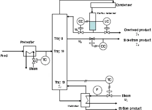
The system being studied is the binary distillation column used to separate ethanol and water.9 Its is a 19 plate distillation column with 12 inch diameter copper column having variable feed and side stream draw-off locations. This example is also used by Chen and Seborg6 to test their method for calculating the uncertain ranges of RGA. A schematic diagram of the binary distillation column is shown in Figure 1.
Figure 1. Schematic diagram of the binary distillation column with diagonal control structure
Table 1 shows steady state values of the column and Table 2 shows system constraints. The following Laplace transfer functions have been identified9 and will be used in this study.
Table 1. Steady state values of binary distillation column
Variable Description Value Units
y1 Overhead mol fraction of ethanol
0.7
y2 The mol fraction ofethanol in the side stream
0.52
y3 Temperature on tray 19 92 °C
u1 Overhead reflux flowrate 0.18 gpm
u2 Side stream draw-off rate 0.046 Gpm
u3 Reboiler steam pressure 20 Psig Table 2. System constraints
Variable Lower
Constraint
Upper Constraint
u1 Overhead reflux flowrate
0.068 0.245
u2 Side stream draw-off rate
0.00694 0.1
u3 Reboiler steam pressure
15.6 34.0
Generally, the RGA of a non-singular square matrix K is a square matrix and defined as:
TK K
RGA 1 (2)
where denotes element by element multiplication. Eq.(2) can be used for 3×3 process and all other systems.
The ijth element of the RGA 10 is:
K K
Kij ij
j i ij
det det
1
(3) Here, Kij is the element on the ith row and jth column of K and Kij is the submatrix that remains after the ith row and jth column of K are deleted.
It is obvious that ij is a function of K, that is
K fij
(4)
Now assume that the uncertainty bounds (lower and upper bounds) for steady state gain, Kij , i=1, 2,
…, n, j=1,2, …, n, are given, then there will be 2n2 constraints for all elements of steady state gains which can be formulated as follows:
b
AX (5) where
X is a vector of size n2×1 containing all elements of K as its elements:
X = [K11 … Knn] T
(6) b is a vector of size (2n2)×1 containing the lower and upper bounds of the corresponding elements of
X.
A isan appropriate matrix of size (2n2)×(n2) satisfying the inequalities in Eq.(5).
Therefore, the lower bound and upper bound of ij can be formulated as the following respectively: Lower Bound:
X
min ij f(X) (7)
Upper Bound:
X
max ij f(X) (8)
Note that ij cannot be determined if det(K) = 0. Therefore, in order to use the above method, the range of det(K) should not include 0. The range of det(K) can be calculated by using the same optimization method.
Optimization algorithm that optimized control performance were used to automate trial and error method. Here, fmincon function in Matlab Optimization Toolbox were used to obtain lower and upper bounds.
3. Results and Discussion
The nominal steady state gain matrix and RGA are given as:
As in Chen and Seborg 6, it is assumed here that the uncertainty for each steady state gain can be expressed as:
ij
The uncertainty ranges for RGA elements calculated via optimization method described in the above Section are given below:
RGA =
The above results indicate that the recommended controller pairing is obvious and unambiguous: (y1-u1, y2 – u2, y3 – u3).
The results obtained via optimization method has wider range for each element of RGA compared to the results from the analytical method. This is because no approximation has been made in optimization method, while Taylor series expansion was used in analytical method. There exists a combination of K which is still within the constraint Eq. (20) and will give the lower and upper bound of relative gains in Eq.(22). This indicates that the proposed method can find more accurate RGA uncertain bounds than the method proposed previously6.
Case 2: α = 0.1
Case 3: α = 0.25
The uncertainty range for RGA cannot be determined as for α = 0.25, the value of det(K) range will include 0 (K can become singular). While using analytical method6, the value of α = 0.5 can still be tolerated.
Closed loop simulation was then performed for the recommended controller pairing (y1 – u1, y2 –
u2, y3 –u3). Table 3 shows the tuning parameters which are obtained via optimization where the sum of absolute errors for setpoint tracking is minimised. The following setpoint changes are used for tuning purpose:
• y1 set-point was changed from 0 to 0.1 at t = 10 min
• y2 set-point was changed from 0 to -0.1 at t = 300 min
• y3 set-point was changed from 0 to -5 at t = 500 min
The output values were recorded for 1000 min simulation time with 1 min sampling time. Therefore, the objective function in the optimization routine is to find a set of controller parameters which will minimise sum of the absolute errors for the specified simulation time.
Table 3. Controller parameters
Controllers Kc τI
y1-u1 0.0871 0.6053
y2-u2 -0.3829 5.1813
y3-u3 6.1938 3.4343
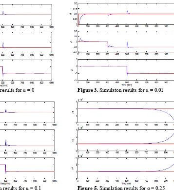
For the nominal values (i.e. no uncertainties), simulation results for set-point changes are shown in Figure 2. In Figure 2, the solid lines represent the controlled variables and the dashed lines represent the set-points. In all the simulations for this example, y1 set-point was changed from 0 to 0.1 at t = 10 min, y2 set-point was changed from 0 to -0.1 at t = 300 min, and y3 set-point was changed from 0 to -5 at t = 500 min. It can be seen from Figure 2 that the control performance is satisfactory.
Simulations are then performed for the arbitrarily altered process gains (which reflect gain uncertainties) as follows:
1 1
1
1 1
1
1 1
1
33 32
31
23 22
21
13 12
11
G G
G
G G
G
G G
G
G (15)
Figures 3 to 5 show the results for three different values of α. Once again, the solid lines represent the controlled variables and the dashed lines represent the set-points. As shown in Figure 5, the
controller settings based on the nominal model cannot guarantee the closed loop stability for α = 0.25. 4. Conclusions
Figure 2. Simulation results for α = 0 Figure 3. Simulaton results for α = 0.01
Figure 4. Simulation results for α = 0.1 Figure 5. Simulation results for α = 0.25 References
[1] Marlin T E 2000 Process Control (Europe: McGraw Hill) [2] Skogestad S and Hovd M 1995 Journal Process Control 5 399 [3] Seki H Naka Y 2006 Ind. Eng. Chem. Res. 45 6518
[4] Bristol E and IEEE Trans 1966 IEEE Trans. Autom. Control 11/1 133
[5] Skogestad S and Postlethwaite I 1996 Multivariable Feedback Control (John Wiley and Sons) [6] Chen D and Seborg D E 2002 AICHE J 48/2 302
[7] Kariwala V Skogestad S and Forbes J F 2006 Ind. Eng. Chem. Res. 45/5 1751
[8] Agustriyanto R and Zhang J 2007 Proc. of the 2007 American Control Conference 5360 [9] Ogunnaike B A Lemaire J P Morari M and Ray W H 1983 AICHE J. 29/4 632