Trajectories of Depression:
Unobtrusive Monitoring of Depressive States by means of
Smartphone Mobility Traces Analysis
Luca Canzian
University of Birmingham, UK
[email protected]
Mirco Musolesi
University College London, UK
University of Birmingham, UK
[email protected]
ABSTRACT
One of the most interesting applications of mobile sensing is monitoring of individual behavior, especially in the area of mental health care. Most existing systems require an interac-tion with the device, for example they may require the user to input his/her mood state at regular intervals. In this paper we seek to answer whether mobile phones can be used to un-obtrusively monitor individuals affected by depressive mood disorders by analyzing only their mobility patterns from GPS traces. In order to get ground-truth measurements, we have developed a smartphone application that periodically collects the locations of the users and the answers to daily question-naires that quantify their depressive mood. We demonstrate that there exists a significant correlation between mobility trace characteristics and the depressive moods. Finally, we present the design of models that are able to successfully pre-dict changes in the depressive mood of individuals by analyz-ing their movements.
Author Keywords
Mobile Sensing; Depression; Spatial Statistics; GPS Traces
ACM Classification Keywords
H.1.2. Models and Principles: User/Machine Systems; J.4 Computer Applications: Social and Behavioral Sciences
INTRODUCTION
According to a recent report by the World Health Organiza-tion [9], in high-income countries up to90% of people who die by suicide are affected by mental disorders, and depres-sion is the most common mental disorder associated with sui-cidal behavior. More generally, depressive disorders do not only affect the personal life of individuals and their families and social circles, but they also have a strong negative eco-nomic impact [28]. In fact, according to a study by the Eu-ropean Depression Association [9],1in10employees in the United Kingdom had taken time off at some point in their working lives because of depression problems. Currently, psychologists rely mainly on self-assessment questionnaires
Permission to make digital or hard copies of all or part of this work for personal or classroom use is granted without fee provided that copies are not made or distributed for profit or commercial advantage and that copies bear this notice and the full cita-tion on the first page. Copyrights for components of this work owned by others than ACM must be honored. Abstracting with credit is permitted. To copy otherwise, or re-publish, to post on servers or to redistribute to lists, requires prior specific permission and/or a fee. Request permissions from [email protected].
UbiComp ’15, September 07-11, 2015, Osaka, Japan c
2015 ACM. ISBN 978-1-4503-3574-4/15/09 $15.00 DOI: http://dx.doi.org/10.1145/2750858.2805845
and phone/in-site interviews to diagnose depression and mon-itor its evolution. This methodology is time-consuming, ex-pensive, and prone to errors, since it often relies on the patient’s recollections and self-representation. As a conse-quence, changes in the depression state may be detected with delay, which makes intervention and treatment more difficult.
Several recent projects have investigated the potential use of mobile technologies for monitoring stress, depression and other mental disorders (see, for example, [25, 6, 31, 24, 36, 1, 5, 39], providing new ways for supporting both patients and healthcare officers [8, 20]. Indeed, mobile phones are ubiqui-tous and highly personal devices, equipped with sensing ca-pabilities, which are carried by their owners during their daily routine [19]. However, existing works mostly rely on periodic user interaction and self-reporting. Our goal is to build sys-tems thatminimizeand, if possible,removethe need for user interaction.
We focus on a specific type of data that can be reliably col-lected by almost any smartphone in a robust way, namely
location information, and we investigate how it is possible
to correlate characteristics of human mobility and depressive state. Indeed, interview-based studies have shown that de-pression leads to a reduction of mobility and activity levels (see, for example, [34]). Previous work has shown the po-tential of using different smartphone sensor modalities to as-sess mental well-being. However, the focus was on the ac-tivity level detected with the accelerometer sensor [31], voice analysis using the microphone [24], colocation using Blue-tooth and WiFi registration patterns [25], and call logs [5]. In this paper instead we focus on the characterization (also from a statistical point of view) and exploitation ofmobility data collected by means of the GPS receivers embedded in today’s mobile phones. More specifically, this work for the first time addresses the following key questions: is there any correla-tion between mobility patterns extracted from GPS traces and
depressive mood? Is it possible to devise unobtrusive
smart-phone applications that collect and exploitonlymobility data in order to automatically infer a potential depressed mood of the user over time?
In order to answer these questions, we need toquantitatively
characterize the movements of the user over a certain time interval and correlate them to anumericindicator of the de-pressed mood of a user. For this reason, we first extract
mobil-ity tracesfor a user and we define and computemobility
pat-terns over time. We then use the questions from the widely-used “PHQ-8” depression test [16, 18, 15] in order to quantify depressive states.
In order to obtain ground truth measurements about the cor-relation of mobility patterns and depressive states, we have developed an Android application for smartphones –
Mood-Traces[27] – that periodically collects the locations of the
users. MoodTraces collects also the answers to8daily ques-tions from the “PHQ-8” depression test that the users are asked to take, concerning the occurrence of specific depres-sive symptoms in the current day. The answers are used to compute a daily integer score for each user ranging from0to
24, which we callPHQ score. For each user, we then analyze how the mobility metrics and the PHQ score vary in time, proving that there exists a significant correlation between them. Driven by these results, we then investigate whether it is possible to predict changes in the PHQ score from vari-ations in the mobility metrics. To achieve this goal, we train and test personalized classification models for each user. An extensive evaluation shows that, for most of the users, these personalized models are able to accurately detect changes in the PHQ score exploiting only mobility metrics. It is worth noting that, after a training phase, these models are able to monitor the depressive state of individuals without requiring a direct interaction with the device. This is particularly im-portant for patients with serious depressive conditions who might not be willing (or, unfortunately, sometimes able) to actively report their condition using the mobile device. More-over, a generic, albeit less accurate, training model built on data collected in pilot studies like this might be used in order to remove the need of a training phase in the deployment of the application.
To summarize, the contribution of this paper is threefold.
First, we design an energy-efficient Android application to
collect mobility data and assess the presence of a depressed mood, and we deploy it and collect data from28users. Sec-ond, we define a set of mobility metrics that can be extracted from the mobility traces of the users and, using the ground truth data collected by means of the Android application, we identify a significant correlation between the changes of such metrics and the variations in the PHQ score. Such a correla-tion ranges from0.336to0.432when the mobility metrics are computed over a period of14days.Third, we train and evalu-ate personalized and general machine learning models to pre-dict PHQ score changes from mobility metrics variations, ob-taining very good prediction accuracies. For example, when the mobility metrics are computed over a period of14days, the general model achieves sensitivity and specificity values of0.74and0.78(respectively), whereas the average sensitiv-ity and specificsensitiv-ity values of the personalized models are0.71
and0.87(respectively).
RELATED WORK
Given the increasing availability of mobility traces extracted by means of GPS phones or WiFi registration records, we have witnessed a growing interest in the investigation of the properties of human movement, with the goal of identifying patterns or developing prediction models [37, 2]. Mobility
and other contextual information are increasingly collected by means of mobile phone sensing applications [7], i.e., by means of sensors (such as GPS, accelerometers, etc.), which are embedded in today’s smartphones.
In particular, in the pervasive and ubiquitous computing com-munity, several projects have investigated the use of smart-phone data for the automatic detection and prediction of psy-chological states and mental health conditions [22, 32, 23, 6].
Stress monitoring using smartphones has been studied in [24, 1, 36, 5]. More specifically, user locations and social inter-actions (through Bluetooth proximity, phone calls and SMS logs) are exploited by the authors of [1] to detect differences between stressful and non stressful periods, showing that be-havior changes can be automatically detected by means of mobile phones.
The detection and monitoring of bipolar disorder by means of mobile technologies are discussed in [10, 11, 29, 12]. The authors in [10] reports the results of a6months trial with6
patients suffering from bipolar disorder, in which they record subjective and objective data (including self-assessments, ac-tivity, sleep, and phone usage) and inform both the patient and clinicians on the importance of the different data items according to the patient’s mood. In [11, 29, 12] the authors describe multiple real-life studies of the use of smartphone based sensors for state monitoring of bipolar disorder. [11] shows initial evidence that relatively simple features derived from location, motion and phone call patterns are a good in-dication of state transitions; [29] analyzes how the episodes of the diseases correlate to the sampled data and suggest that personalized models are better suited to detect early signs of the onset of a bipolar episode; [12] studies the detection of state changes, achieving a precision and recall of96% and
94%, respectively, and state recognition accuracy of80%.
To the best of our knowledge this work for the first time demonstrates that it is possible to devise metrics that can be used to capture the correlation between mobility patterns ex-tracted from GPS traces and depressive mood. Moreover, our paper differentiates from the above cited literature in a num-ber of different ways.First, the works in [24, 23, 6, 1, 36, 5] focus on mood or stress detection and not on the analysis and prediction of variations of the depressive states of individuals.
20
Figure 1:THISTis the duration of the interval over which we
compute the metrics, whereasTHORrepresents how much in
advance we compute the metrics. In other words, with respect to the example in the figure, we try to answer the following question: is there a relationship between the user mobility behavior from 20February until25 February and the PHQ score result obtained on day28February?
consequence, our technique can also be applied to monitor the PHQ score of a user that does not suffer from any form of depression (i.e., having a low PHQ score), and for an early depression diagnosis in case the condition of the user wors-ens.
OUR APPROACH
The key question of this paper, which is illustrated in Fig. 1, is whether the mobility behavior of an individual can give information about his/her current depressive state, which is quantified by a PHQ score. In order to answer this question, we first need to introduce the key definitions and notations that we use in this work. In the following we provide a formal definition ofmobility traces and we define a set ofmobility metrics, i.e., a set of statistical summaries characterizing the movement of individuals.
Formal Definition of Mobility Traces
We consider themobility traceof a user as a sequence of stops and moves. This is a widely used definition of mobility trace (see for example [38]). A stop represents a geographic loca-tion in which the user spends a certain interval of time. For-mally, we define astop place(shortly,place) as a tuple:
P l=hID, ta, td, Ci, (1)
whereID is an identifier,ta is the time of arrival,td is the
time of departure, andC is a latitude-longitude pair. For a specific user we define the mobility traceM T(t1, t2)for the time interval[t1, t2]as the sequence of places visited by that user during that time interval:
M T(t1, t2) = (P l1, P l2, . . . P lN(t1,t2)), (2)
whereN(t1, t2)is the total number of visited places in the interval[t1, t2]. The time references satisfy the following in-equalities: ta
, correspond to periods of time in which the user is moving from one place to another. Whenever we do not specify the time interval of a mobility trace, we im-plicitly consider a time interval equal to the period of study. 1We use the subscriptito denote a parameter of thei-th place. For
example,ta
i represents the time of arrival of the placeP li.
Mobility Metrics
In this work, the mobility traces are used to compute a set of
mobility metrics, which represent an aggregate information
about the user movements. The considered metrics have been designed to capture behavioural patterns associated with de-pression such as reduced mobility [34] and, more generally, limited willingness of performing different activities, which usually involve movements to various locations [18]. It is quite interesting to note that the proposed metrics are also able to capture behavioral characteristics that might not be visible through traditional questionnaire-based methods. We consider the following mobility metrics, which are associated to a specific user and time interval[t1, t2].
1) The total distance coveredDT(t1, t2). We formally
de-fine this distance as follows:
DT(t1, t2) = latitude-longitude pairsCiandCi+1.
2) The maximum distance between two locations
DM(t1, t2). It represents the maximum span of the area cov-ered in the interval[t1, t2]. More formally:
DM(t1, t2) = max
i,j∈{1,...,N(t1,t2)}d(Ci, Cj). (4)
3) The radius of gyrationG(t1, t2). This metric is used
to quantify the coverage area and is defined as the deviation from the centroid of the places visited in the interval[t1, t2] [13]. We weight the contribution of each place by the time spent in that place. LetTi = tdi −tai the time spent in the
i-th place,T˜ =PN(t1,t2)
i=1 Tithe total time spent in different
places, andCcenthe coordinates of the centroid of the places
visited in the interval[t1, t2], then:
4) The standard deviation of the displacements σdis.
With “displacement” we refer to the distance between
one place and the subsequent one. Let Ddis =
1
all the places visited by the user during the period of study, we assign the label “home” to the cluster in which the user was found most often at02:00,06:00and20:30during weekdays. LetCHthe coordinates of such a cluster, then:
DH(t1, t2) = max
6) The number of different places visitedNdif(t1, t2). Let
1ijthe indicator function, which is equal to1ifIDi=IDj,
otherwise it is equal to 0. The we can formally define Ndif(t1, t2)as:
7) The number of different significant places visited
Nsig(t1, t2). We assign the label “significant place” to each of the10most visited places among all the places visited by the user during the period of study. Nsig(t1, t2)quantifies how many of these significant places are visited in the inter-val[t1, t2]. LetIDs1, . . . , IDs10the IDsof the significant
ric with the goal of quantifying how different the places vis-ited by the user during the time interval[t1, t2]are with re-spect to the places visited by the user during the same time interval in other days. To formally define this metric we need to introduce some further notation. Given the mobil-ity traceM T(t1, t2), we define the augmented mobility trace M T(t1, t2)as the mobility trace in which the gaps between places are filled with “mobility places”, and we denote by IDmtheIDsof these places.
We define the difference functionft(M T
1, M T2)between
where we use the notation IDi,t to denote the ID of the
place belonging to the i-th trace and visited by the user at time t. Basically, for two overlapping mobility traces, ft(M T
1, M T2)checks whether the place at time instantt is different for the two traces.
Now we can define the average differencef(M T1, M T2) be-tweenM T1andM T2as the fraction of the overlapping time in which the places inM T1are different from the places in M T2:
We define the translated augmented mobility trace
M Tt(t1, t2) as the mobility trace that is obtained from M Tt(t1, t2) by translating all the times in advance by an amount equal tot.
Lettinitandtf inbe the time of arrival and the time of
depar-ture of the first and last places visited by the user in the period of study, respectively. LetT be the length of one day,n1the number of (whole) days elapsed fromtinittot1, andn2the number of (whole) days elapsed fromt2totf in. Finally, we
define the routine index as:
R(t1, t2) = 1 difference between the mobility behavior of the user in[t1, t2] and the mobility behavior of the same user in other days in the same (daily) time interval. Notice that0≤R(t1, t2)≤1.
Finally, we would like to remark the fact that these metrics are able to capture also the absence of movement, which might be associated to specific mental health states, for example, a person that stays at home for subsequent days or that do not go far from his/her home because of his/her depressive mood.
MOODTRACES APPLICATION
Overview
MoodTraces is an Android application for mobile phones that automatically samples phone’s sensors to retrieve the current location, which is represented by a time reference, a longi-tude value, and a latilongi-tude value. Additional information about the phone usages and user activities extracted using the An-droid API are also collected, but they are not analyzed di-rectly in this work, given its specific focus on mobility pat-tern analysis. Activity information is used to optimize the sampling process as discussed below. In addition to sensor based data, MoodTraces collects the answers that the users provide to daily questionnaires. It is worth noting that this application collects information about the user mood only to get the ground-truth data. All the collected data is sent via a secure transmission protocol to a secure server located at our institution. We exploit the asynchronous delay-tolerant data transfer strategy of the ES Data Manager Library [32, 21] to transmit the collected data in an energy-efficient way and to avoid any cost on participating users.
Location Collection Process
One of the key challenges for mobile sensing applications is their energy use and impact on battery life. Among all the data collected by MoodTraces, GPS-based location data are by far the most expensive in terms of energy consumption [3, 26]. In order to limit the energy impact of the location data collection, we exploit the collected activity data2 to trigger location sampling only when the user moves from one place
2We collect activity data with a sampling rate of
1minute. However,
M U
S
Two dynamic activities with high confidence
Location changed significantly
Location did not change significantly
Two "still" with high confidence or location
did not change
(a) State-based sampling rate.
GPS network
Long time since last GPS attempt
Not able to get GPS location
(b) State-based provider.
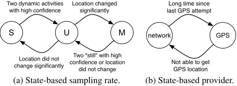
Figure 2: State machines to select the location sampling rate and the location provider.
to another. Our approach is represented by the state machine in Fig. 2a.
The three states that we consider and the corresponding loca-tion sampling rates adopted are described in the following.
Static (S): in this state we never sample location data. This
state corresponds to all the situations in which we are confi-dent that the user is remaining in the same place (e.g., during working hours a user may remain for an extended period in-side the building in which he/she works; it is not necessary to sample location data continuously in this case).
Moving (M): in this state we sample location data with a
sam-pling rate ofTs = 5minutes. This state corresponds to the
situations in which we are confident that the user is moving from one place to another (e.g., when the user moves from his/her working place to his/her home).
Undecided (U): as soon as we enter this state we get the user
location, and then we get another user location afterTs = 5
minutes. Based on the distance between the two locations, we decide whether to transit to theSor to theMstate. This state corresponds to all the situations in which we are not sure whether the user is moving from one place to another (e.g., the phone may detect that the user is walking, but we are not sure whether the user is walking from his/her working place to his/her home, or whether the user is walking from one office to another office at his/her workplace). When Mood-Traces is installed, and whenever the smartphone is rebooted, we initialize the state toU.
We transit from S to Uwhenever two consecutive activity samples indicate that the user is performing a “dynamic ac-tivity” (i.e., in vehicle, on bicycle, on foot, running, walking) with a confidence level larger thanPth = 50%. We transit
fromMtoUwhenever either 1) we get two consecutive lo-cation samples whose distance is smaller thandth= 250m;
or 2) two consecutive activity samples indicate that the user is “still” with a confidence level larger thanPth= 50%.
Fi-nally, fromUwe transit toMif the two location samples that we collect inside theUstate are more thandth= 250m apart,
otherwise we transit toS.
In addition to the sampling rate, the choice of the “location provider” has also an important impact on the energy con-sumption. Indeed, in Android it is possible to sample location data by using either the “GPS provider”, which is accurate
but energy-demanding and limited in indoor environment, or the “network provider”, which provides less accuracy but is much less energy-demanding than the GPS provider. In order to trade-off accuracy with energy consumption, MoodTraces implements the simple state machine represented in Fig. 2b. Each state represents the provider that will be used in case MoodTrace requests a location sample. By default, in order to have accurate location we use the GPS provider. If we do not receive any location update in1minute after a request (e.g., the GPS receiver is not able to track the GPS signal because the user is moving using a subway), then we switch to the net-work provider. We switch back to the GPS provider after30
minutes we entered the network provider state. MoodTraces subscribes also to a “passive location provider”, meaning that it passively receives location updates when other applications or services request them, independently of the states of the two state machines represented in Fig. 2.
Questionnaire Collection Process
The PHQ-9 is a widely used and extensively studied9-item questionnaire for assessing and monitoring depression sever-ity [16, 18, 15]. A systematic review of the PHQ-9 is reported in [18]. It shows that, in19studies, the PHQ-9 achieves sensi-tivity values ranging from0.77to0.88, and specificity values ranging from0.88to0.94. As a comparison, [4] identifies12
studies that address the performance of the Hospital Anxiety and Depression Scale (HADS) and reports a mean sensitivity of0.83and a mean specificity of0.79, and similar sensitiv-ity and specificsensitiv-ity values are achieved by the General Health Questionnaire (GHQ).
The PHQ-8 is an8-item questionnaire that omits the ninth item of the PHQ-9 questionnaire. [18] reports correlation values of0.998 and0.997in two different studies between PHQ-9 scores and PHQ-8 scores, and [16] suggests to use the PHQ-8 instead of the PHQ-9 in clinical samples in which the risk of suicidality is felt to be extremely low or if data is being gathered in a self-administered fashion. Since both of these conditions are met in our study, and because of its brevity and its structure, a PHQ-8 based daily questionnaire is used in MoodTraces to assess the presence of a depressed mood and how this varies in time.
The PHQ-8 is composed of8questions: for each of them the participant is asked to report the frequency of the occurrence of a specific depressive symptom during the last2 weeks. Based on the provided answers, each question is associated with a score between0and3. The finalPHQ scoreis com-puted by adding the contributions of all questions; hence, it ranges from0to24. Cut points of5,10,15and20are con-sidered to diagnose mild, moderate, moderately severe and severe levels of depressive symptoms, respectively [17, 16, 18, 15]. As stated in [18], these categories were chosen both for pragmatic reasons, in that the cut points of5,10,15, and
to [18]. Given the fact that the accuracy of the PHQ-8 test is comparable to the accuracy of other tests, the main reason that led us to the adoption of the PHQ-8 test is its brevity and its structure that allow for the design of a simple daily “yes-no” questionnaire in which the user is asked whether each of the depressive symptoms occurred during that day. In this way, the PHQ score for a certain day can be computed by looking at the answers provided during the previous two weeks and computing the frequencies for each depressive symptom.
During each day the questionnaire is available from16:00 un-til2:00of the subsequent day.3,4 A notification at16:00 in-forms the user that the questionnaire is available, following by other notifications at20:00and23:30in case the user has not completed the questionnaire by that time. The question-naire takes less than1minute to complete and can be com-pleted in multiple sessions. Notice that we collect also the an-swers to the questionnaires that are only partially completed.
According to the best practice in survey design [30, 35, 33] we collect the completion time for each provided answer and the questionnaire includes a trap question (i.e., a question having a known answer), asking whether the user is at home or at work. The validity of the answer is checked through-out the collected location data. The answer completion times and the trap questions allowed us to verify the quality of the collected data and to discard non reliable questionnaires.
Recruitment Process
MoodTraces has been available for the general public for free in the GooglePlay Store [27] since September3,2014, and, at the time of writing of this paper, it is still available. The study presented in this paper refers to the data collected from September3,2014, to June14,2015. In this period we had a total of184installs and46users had MoodTraces running in their phones at June14,2015.
At the beginning MoodTraces has been used only by few re-searchers with the goal of fixing bugs, tuning parameters, and adding features to improve the user experience. We have ad-vertised our study starting from the end of November, exploit-ing different resources: academic mailexploit-ing lists, Twitter, Face-book, Reddit, and charities. To promote the application and to give incentives to the users to reply to the questionnaires, we committed to select (through a lottery) one winner of a Nexus5mobile phone and five winners that have received a
10pounds Amazon voucher each among all the participants that have completed the daily questionnaire at least50times in a two-month span. Finally, we remark that we received the full approval of the Ethics Review Board of our institution before starting the recruitment process, and that all the doc-umentation, including the consent form and the information sheet for the participants, are available on request.
DATA PROCESSING
In this section we describe how we processed the data to cal-culate the PHQ score and the mobility metrics for each user
3We chose to make the survey available from late afternoon because
it asks whether depressive symptoms have occurred in the current day, hence it cannot be taken at the beginning of the day.
4
All the times are in the user local time.
on a daily basis. It is worth noting that this procedure was dis-cussed and approved with colleagues that are leading experts in suicidal prevention studies and in clinical practice.
PHQ Score Computation
For each user, we exploit the answers to the daily question-naires that the user provides in order to compute his/her PHQ score on a daily basis.
First, in order to improve the reliability of the collected an-swers, we void 1) the questionnaires for which the trap ques-tion has been replied erroneously, and 2) the quesques-tionnaires that are replied too quickly, as in [35] and [33] we identify these questionnaires as the10% questionnaires with lowest Speeder Index. To compute the Speeder Index we first cal-culate the median completion time for each answer across all the questionnaires of all the users. Then, to each answer we assign a value of1if the completion is at least equal to the me-dian, otherwise we assign a value equal to the ratio between the answer completion time and the median completion time. Finally, for each questionnaire the Speeder Index is computed as the average value of all the provided answers.
Second, to compute the PHQ score on a given dayxwe re-trieve all the questionnaires that have been submitted from dayx−13until dayxand we count how many times each de-pressive symptom occurred in this time interval. Since some answers are missing for some days (e.g., because the users did not submit the questionnaire or submitted an incomplete questionnaire), we deal with missing answers by using a lin-ear interpolation to compute the occurrence frequency of the corresponding symptom. For example, if in a 2-week period the user replies12times to a specific answer indicating that the corresponding symptom occurred6times, then we assign an occurrence frequency for that symptom equal to 7 days over14. The linear interpolation is adopted only if the user replies to at least80% of the answers, otherwise we do not compute a PHQ score for the corresponding day. Our ap-proach follows the current practices in the area, as it is pos-sible to observe in previous other studies based on PHQ-9, in which missing values were replaced with the mean value of the remaining items if the number of missing items was below20%[15, 18].
Third, based on the occurrence frequency we assign the ap-propriate score to each depressive symptom (see [18]), and the PHQ score is computed as the sum of the scores of all depressive symptoms.
Finally, to remove cyclicity effects, from the computed PHQ score we subtract the average PHQ score obtained by that user in that day of the week. In order to simplify the presentation, in the remainder of the paper we use the terms PHQ score to indicate the deviations from the average values (with the exception of Fig. 3 that shows the histograms of the real PHQ scores).
Mobility Traces and Mobility Metrics Computation
places. Indeed, when the user remains in a place for an ex-tended period of time MoodTraces enters the stateSas dis-cussed above. If the user performs some minor movements (e.g., walking from one office to another office at his/her workplace), MoodTraces enters the U state and then goes back to S, because it realizes that the user did not move more thandth = 250m away from the previous place. On
the other hand, if the user performs major movements then MoodTraces enters theMstate after transiting on theUstate. Hence, by looking at the evolution of the state machine we can identify the intervals in which the user stops in a place from the periods in which the user moves.
Since we are not interested in identifying two locations that are in close proximity as different places (e.g., two different offices in the same building), we register the departure from a place if and only if both the transitionS→Uandthe tran-sitionU→Moccur; in this case the departure timeTdis set
equal to the time in which the transitionS→Uoccurs. Anal-ogously, we register the arrival in a place if both the transition
M→Uandthe transitionU→Soccur, and the arrival time Ta is set equal to the time in which the transitionM→ U
occurs. As for the coordinates of the place, we set them equal to the centroid of all locations collected in the time interval
[Ta, Td]having an accuracy of at leastd
acc= 200m. Since
the thresholddth = 250m is used to determine the
transi-tion from the stateU, the geographic area corresponding to a place can be approximately quantified by a circle centered in the coordinates and having a radius ofdth= 250m.
Similarly to the case of the questionnaire collection process, also the location collection process is prone to missing values. Let[t, t]a time interval in which location data are not avail-able due to external factors (e.g., the phone is switched off or the location services are disabled). We deal with this situation by assigning the time interval[t, t]to a stop place if the last location collected before the timetis in close proximity to the first location collected after the timet, i.e., if their minimum distance is belowdth= 250m (this is the case, for example,
of a user that switches off his/her phone before sleeping, and switches it on the next morning). Otherwise that interval will be associated to user movements (this is the case, for exam-ple, of a phone with a fully depleted battery during a trip). However, to avoid to use low quality data, we do not compute the mobility trace (and, as a consequence, the mobility met-rics) associated to a time interval[t1, t2]such that the sum of the periods in which location data are missing is larger than half the target interval, i.e., t2−t1
2 .
Finally, notice that many places in which a user stops corre-spond to geographic locations that the user visits more than once during the period of study (e.g., home, work, bus stop, etc.). It is convenient to use the same ID and coordinates for the places corresponding to the same geographic location. To achieve this goal we adopt the following simple clustering al-gorithm:
1. FindP liandP lj such thatIDi =6 IDj andd(Ci, Cj) =
minn6=m{d(Cn, Cm)}, where d(Cn, Cm) denotes the
dis-tance between the coordinates of the placesP lnandP lm;
2.Ifd(Ci, Cj)< daccthen assignIDj←IDi,Ci←y, and
Cj ←y, whereyis the centroid of all locations collected in
the time intervals[Ta
i, Tid]and[Tja, Tjd]having an accuracy
of at leastdacc= 200m;
3.Iterate1.and2.until convergence.
At each step the above algorithm finds, among all the stop places, the two places that are closest to each other. If they are in close proximity (closer thendacc = 200m) they are
given the sameIDand their centroid is recomputed, other-wise the algorithm terminates. Convergence is guaranteed because the algorithm iterates a maximum ofN(t1, t2)−1 times, after which all places are clustered under the sameID. Once we get the mobility trace of a user, the mobility met-rics for a certain time interval[t1, t2]can easily be computed adopting Eqs. (3) to (9) and (12). Finally, as we did for the PHQ scores, in order to remove cyclicity effects, from each computed mobility metrics we subtract the average mobility metric obtained by that user in that interval in that day of the week.
Combining Mobility Metrics and PHQ Scores
For each user, we compute the time series of the PHQ scores and of the mobility metrics,
PHQ= P HQ1, P HQ2, . . . , P HQN
DT(THIST, THOR) = DT1(THIST, THOR), . . .
DM(THIST, THOR) = DM1 (THIST, THOR), . . .
..
. (13)
whereN is the total number of days the user utilized Mood-Traces in the period of study,P HQi is the PHQ score
asso-ciated to thei-th day since the user downloaded MoodTraces, andDi
T,DMi , etc., are the mobility metric associated to the
PHQ scoreP HQi. We associate each PHQ score to the
mo-bility metrics through the use of thetime historyTHIST and
thetime horizonTHORparameters, which define the interval
over which the mobility metrics are computed, as illustrated in Fig. 1. The parameterTHIST represents the length of the
interval over which the mobility metric is computed, whereas THOR represents how much in advance with respect to the
PHQ score the mobility metric is computed. Hence, for each mobility metric we must compute one sequence of values for each considered combination of the parametersTHIST and
THOR.
We define the vector
P HQi, Di
T(THIST, THOR),
Di
M(THIST, THOR), . . . as the i-th instance. For each
user, we remove the instances for which either the PHQ score or the mobility metrics cannot be computed. Finally, we exclude from the study all the users having less than Ninst = 20 instances. As a consequence of this filtering
procedure, the evaluation presented in this paper is generated from a dataset of28users, which is briefly described in the following.
0 1 2 3 4 5 6 7 8 9 10 11 12 13 14 15 16 0
1 2 3
4 Histogram of the average PHQ scores of the users
Average PHQ score
Number of users
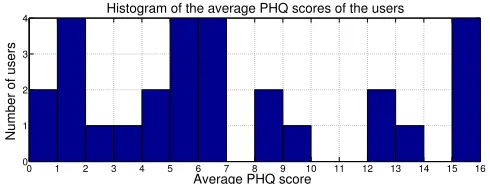
Figure 3: Histograms of the average PHQ score of the users.
Many of these are linked to the academic environment (7 stu-dents,3PhD students, and7researchers/lecturers), but there are also individuals working in the private sector, artists, and retired people. The average age is31years old. On average each user has been monitored for71days, and we were able to compute63PHQ scores for each user. Figure 3 shows the histogram of the average PHQ scores of the users. Most of the users do not suffer, on average, of depressive problems (average PHQ score below5), or they suffer of mild depres-sive symptoms (average PHQ score from5to10). However, there are also some users suffering of moderate (average PHQ score from 10to15) and moderately severe (average PHQ score from15to20) depressive symptoms. These users ex-perience also peaks on the daily PHQ score overpassing the severe depression cut point value20.
EVALUATION
In this Section we analyze the data collected by means of MoodTraces. We first analyze how the mobility metrics and the PHQ score of each user jointly vary in time, proving that there exists a significant correlation among them. Then we train and test personalized regression and classification mod-els for each user to investigate whether it is possible to pre-dict changes in the PHQ score from variations in the mobility metrics.
Correlation Analysis
We exploit the sequences defined by Eq. (13) to analyze the correlation5between each mobility metric and the PHQ score, for each user and for different values of the time history pa-rameterTHIST, which is measured in days. We also compute
the p-value associated to each correlation value, represent-ing the probability of gettrepresent-ing a correlation as large as the ob-served value by random chance (i.e., when the true correlation is zero). For this analysis we set the time horizonTHOR= 0
days, i.e., the last day of the time interval over which we com-pute a specific mobility metric is equal to the day in which we compute the associated PHQ score.
Table 1 shows the average values (among the users) of the absolute correlations and p-values, for each mobility metric and forTHIST = 1day (i.e., the mobility metrics are
com-puted over the same day of the corresponding PHQ score) and THIST = 14 days (i.e., the mobility metrics are computed
considering a time span of two weeks before the day of the
5In this work we consider the Pearson correlation [40], which is
usually adopted to quantify linear dependences between variables.
Mobility metric TAverage abs. correlation Average p-value
HIST= 1 THIST= 14 THIST= 1 THIST= 14
DT 0.159 0.402 0.401 0.095
DM 0.152 0.432 0.425 0.069
G 0.160 0.343 0.422 0.197
σdis 0.147 0.417 0.431 0.088
DH 0.199 0.358 0.297 0.168
Ndif 0.191 0.360 0.335 0.157
Nsig 0.201 0.336 0.385 0.181
R 0.227 0.368 0.262 0.138
Table 1: The averages of the absolute values of the correla-tions and of the p-values for different mobility metrics, for THIST = 1day andTHIST = 14days.
corresponding PHQ score). We consider the absolute value of the correlation because it represents an ordinal measure of how strong the relationship between the mobility metric and the PHQ score is, hence it is reasonable to compute its aver-age (this does not hold for the “signed correlation”, because strong negative and positive dependencies would compensate each other by computing the average).
ForTHIST = 1the average correlations6range from0.147
(associated to the metric σdis) to 0.227 (associated to the
metric R). Though these values are significantly different from0, since the number of instances for each user is not extremely large the corresponding average p-values are quite large. Indeed, usually a correlation value is considered sig-nificant only if the corresponding p-value is smaller than the significance levelα= 0.05, but in our case the minimum p-value forTHIST = 1is0.262. ForTHIST = 1“low level”
metrics such as the total distance coveredDT or the
maxi-mum distance between two locationsDM have a smaller
av-erage correlation than the metrics that capture semantic in-formation about the visited places, such as the number of different significant places visitedNsigor the routine index
R. Interestingly, this situation is reversed forTHIST = 14.
This suggests that low level distance-based metrics such as DT andDM require the observation of the user mobility
be-havior for longer time intervals than metrics that incorporate some semantic about the visited places. However, for suffi-ciently long time intervals, they can provide stronger clues about the depressive state of the user. With the increase of THIST from 1 to14 days the average correlation for each
mobility metrics increases (ranging now from0.336forNsig
to0.432 forDM) and, as a consequence, the corresponding
p-values decrease.
This aggregate analysis summarized in Table 1 provides in-teresting insights about the correlation between PHQ scores and mobility metrics, but it does not provide a complete un-derstanding of the strength of the correlation at individual level. For this reason, we now investigate the correlations and p-values in a non-aggregate form, by plotting the his-tograms of their values forTHIST = 1andTHIST = 14.
Due to space constraints, it is not possible to show the his-tograms for all mobility metrics. Hence, we choose to
con-6
Histograms correlation and p values for different metrics (T
20 Maximum distance DM
p values
Figure 4: Histograms of the correlation and of the p-values forTHIST = 1day.
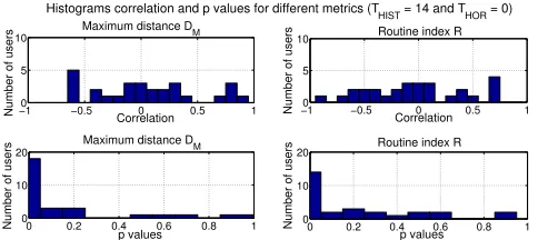
Histograms correlation and p values for different metrics (T
HIST = 14 and THOR = 0)
Figure 5: Histograms of the correlation and of the p-values forTHIST = 14day.
sider only the maximum distance between two locationsDM,
whose average correlation is the second worst of all metrics forTHIST = 1and the best forTHIST = 14, and the routine
indexRthat, on the other extreme, has the best average cor-relation forTHIST = 1. The histograms of the other mobility
metrics are very similar to the histograms of the two selected metrics.
Fig. 4 shows the histograms of the correlation and of the p-values forTHIST = 1day. The histograms of the
correla-tion associated toDM (top-left subfigure) and toR(top-right
subfigure) are distributed closely around0, and the associ-ated p-values (bottom-left and bottom-right subfigures) are quite large: there are only3 users forDM and2 users for
Rhaving a p-value lower thanα = 0.05, corresponding to the first bin of the p-value histogram. Fig. 5 shows that for THIST = 14days the correlation values for both mobility
metrics are distributed more uniformly. It is important to re-mark that different users react differently to changes in their moods, for example an increase in the PHQ score is associ-ated to smaller travelled distances for some users (those for which the correlation between PHQ score andDM is
nega-tive) and larger travelled distances for others (those for which the correlation is positive). This suggests that personalized models, instead of general ones, should be used to monitor the depressive state of an individual using his/her mobility traces. Quite interestingly, Fig. 5 shows that there are18
users forDM and14users for R for which the p-value is
lower thanα= 0.05, meaning that the corresponding corre-lation can be considered significant.
Histograms sensitivity for different values of T
HIST (THOR = 0)
Figure 6: Histogram of the sensitivity, forTHIST = 1,7, and
14days.
Histograms specificity for different values of THIST (THOR = 0)
0 0.5 1
Figure 7: Histogram of the specificity, forTHIST = 1,7, and
14days.
Prediction Analysis
The fundamental question that has driven this study is whether it is possible to monitor and diagnose a depressed mood by looking at the mobility trace collected from a smart-phone of an individual. To answer to this question we set up the following analysis with the collected data. For each user and for each instance we compute a “label” in the following way: the label is equal to1if the PHQ score is larger that the average PHQ score of that user plus one standard deviation, otherwise the label is equal to0. A label equal to1 corre-sponds to the situation in which the user has a a PHQ score that is significantly larger than its usual value. Our goal is to develop models that are able to detect this situation. For each user, we train and test a personalized Support Vector Machine (SVM) classifier with a Gaussian radial basis function kernel [14]. In order to fully exploit the limited number of instances available for each user, we adopt a leave-one-out cross vali-dation approach for training and testing. Moreover, for each training test we adopt again leave-one-out cross validation in order to optimize the value of the SVM penalty parameterC. We vary such a parameter using the exponentially growing sequenceC= 2−5,2−3, . . . ,25.
To quantify the performance of the classification models we consider two metrics: 1) thesensitivity(or true positive rate), i.e., the fraction of1labels that are correctly classified; and 2) thespecificity(or true negative rate), i.e., the fraction of
0labels that are correctly classified. In our first analysis we show the histograms of the sensitivity and specificity, for dif-ferent values ofTHIST and forTHOR = 0. The results are
shown in Figs. 6 and 7. AsTHIST increases, the distributions
of the values of both the sensitivity and the specificity move
closer to1. On one extreme, withTHIST = 1 day many
2 4 6 8 10 12 14 0
0.2 0.4 0.6 0.8 1
Average sensitivity and specificity vs. T
HIST (THOR = 0)
T
HIST [days]
Probability Sensitivity personalized models Specificity personalized models Sensitivity unique model Specificity unique model
Figure 8: Average sensitivity and specificity values vs. THIST, forTHOR= 0days.
On the other extreme, withTHIST = 14days most of the
trained models achieve very large sensitivity and specificity values. This means that, for most of the users, these person-alized models are able to detect periods in which the users experience an unusual depressed mood (this is linked to the sensitivity), and at the same time they generate very few false alarms (this is linked to the specificity). Notice that for all the users the specificity values are larger than the sensitivity values: this is not surprising because we are trying to detect unusual PHQ scores for each users, hence the datasets are unbalanced (they contain more 0 labels than 1 labels) and, as a consequence, in order to minimize the mis-classification probability, the trained SVM models are biased toward the predictions of the0labels.
Next we investigate how the average (among the users) sen-sitivity and specificity values vary with the time interval THIST, forTHOR = 0. The results are showed in Fig. 8.
Average sensitivity and specificity values are associated with a confidence bar, which covers an interval of two standard de-viation around the average value. Fig. 8 shows also the sen-sitivity and specificity value of a generic SVM model, which is trained and tested with the same modalities of the person-alized models, but it exploits all the data collected from all the28users. Both the average sensitivity and specificity of the personalized models and the sensitivity and specificity of the unique model rise with the increase ofTHIST, and reach
large values forTHIST = 14days. We notice that
personal-ized models achieve better performance that the unique gen-eral model, confirming the insights derived from the correla-tion analysis. However, the good performance of the unique general model demonstrates the feasibility of this alternative approach, which has the advantage that it does not require the collection of labeled data from each user for training pur-poses, and this might increase the actual usability and accep-tance of the proposed prediction tools. This represents an interesting trade-off to explore. For example, a model trained on all the data can be adopted when personalized data are not available, e.g., when a user installs an application relying on these mechanisms for the first time.
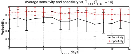
In our final analysis we fix the value of the time interval THIST to14days and we vary the parameterTHOR; the
av-erage sensitivity and specificity values obtained (along with the corresponding confidence bars) are represented in Fig. 9. As expected, the average sensitivity and specificity val-ues decrease asTHORincreases. This is not surprising since
0 2 4 6 8 10 12 14 0
0.2 0.4 0.6 0.8 1
Average sensitivity and specificity vs. T
HOR (THIST = 14)
THOR [days]
Probability
Sensitivity Specificity
Figure 9: Average sensitivity and specificity values vs. THOR, forTHIST = 14days.
THORrepresents the prediction horizon (see Fig. 1), i.e., how
much in advance we try to predict the change in the PHQ score of the user. However, it is surprising that the decay is very slow. Indeed, the average sensitivity and specificity are quite large even if we try to predict changes in the PHQ score14days in advance, which is for example the time span over which depressive symptoms are evaluated in the PHQ-8 test (and in many other standard test to diagnose depression). This means that the considered mobility metrics might iden-tify early signs that can be exploited for an early detection of depressed moods.
CONCLUSIONS
In this work we have demonstrated that it is possible to ob-serve a significant correlation between mobility patterns and depressive mood using data collected by means of smart-phones. We have also shown that it is possible to develop in-ference algorithms as a basis for unobtrusive monitoring and prediction of depressive mood disorders.
We believe that this work represents an important starting point in this area and can be used as a basis for more application-oriented projects in the area of digital mobile in-terventions. For example, the techniques for automatic detec-tion of depressive state presented in this work can be used for building systems for automatic interventions, both through technology (e.g., phone calls from healthcare officers) or tra-ditional physical interactions. Moreover, the focus of this pa-per is on a specific modality, i.e., GPS location, but the results of this work can be indeed exploited to build a more refined system based on the analysis of data extracted by means of other sensors, such as accelerometers, and other sources of information, such as call and SMS logs. Finally, we plan to use the current application (or an extended version) in future studies that will focus on specific populations, such as indi-viduals that have been clinically diagnosed as depressed.
ACKNOWLEDGEMENTS
The authors would like to thank all the participants of this study. Prof. Rory O’Connor and Dr Paul Patterson pro-vided an invaluable contribution to the study, in particular for the design of the experiments. This work was supported through the EPSRC grant “Trajectories of Depression: In-vestigating the Correlation between Human Mobility Pat-terns and Mental Health Problems by means of Smartphones” (EP/L006340/1) and partially by the “LASAGNE” Project,
Contract No. 318132 (STREP), funded by the European
REFERENCES
1. Bauer, G., and Lukowicz, P. Can smartphones detect stress-related changes in the behaviour of individuals?
InProceedings of PERCOM ’12 Workshops(March
2012), 423–426.
2. Baumann, P., Kleiminge, W., and Santini, S. How Long Are You Staying? Predicting Residence Time from
Human Mobility Traces. InProceedings of MobiCom
’13(2013), 231–234.
3. Ben Abdesslem, F., Phillips, A., and Henderson, T. Less is More: Energy-efficient Mobile Sensing with
Senseless. InProceedings of MobiHeld ’09(2009), 61–62.
4. Bjelland, I., Dahl, A. A., Haug, T. T., and Neckelmann, D. The validity of the Hospital Anxiety and Depression Scale.Journal of Psychosomatic Research 52, 2 (2001), 69–77.
5. Bogomolov, A., Lepri, B., Ferron, M., Pianesi, F., and Pentland, A. S. Pervasive stress recognition for sustainable living. InProceedings of PERCOM ’14
Workshops(March 2014), 345–350.
6. Burns, M. N., Begale, M., Duffecy, J., Gergle, D., Karr, C. J., Giangrande, E., and Mohr, D. C. Harnessing context sensing to develop a mobile intervention for depression.Journal of Medical Internet Research 13, 3 (August 2011).
7. Campbell, A. T., Eisenman, S., Lane, N., Miluzzo, E., Peterson, R., Lu, H., Zheng, X., Musolesi, M., Fodor, K., and Ahn, G.-S. The rise of people-centric sensing.
IEEE Internet Computing 12, 4 (July 2008), 12–21.
8. Donker, T., Petrie, K., Proudfoot, J., Clarke, J., Birch, M.-R., and Christensen, H. Smartphones for smarter delivery of mental health programs: a systematic review.
Journal of Medical Internet Research 15, 11 (2013).
9. European Depression Association. IDEA: Impact of Depression at work in Europe Audit, September 2012.
10. Frost, M., Doryab, A., Faurholt-Jepsen, M., Kessing, L. V., and Bardram, J. E. Supporting Disease Insight Through Data Analysis: Refinements of the Monarca Self-assessment System. InProceedings of UbiComp ’13(2013), 133–142.
11. Gr¨uenerbl, A., Oleksy, P., Bahle, G., Haring, C., Weppner, J., and Lukowicz, P. Towards smart phone based monitoring of bipolar disorder. InProceedings of
mHealthSys ’12(2012).
12. Gr¨uenerbl, A., Osmani, V., Bahle, G., Carrasco, J. C., Oehler, S., Mayora, O., Haring, C., and Lukowicz, P. Using Smart Phone Mobility Traces for the Diagnosis of Depressive and Manic Episodes in Bipolar Patients. In
Proceedings of AH ’14(2014).
13. Hoteit, S., Secci, S., Sobolevsky, S., Pujolle, G., and Ratti, C. Estimating Real Human Trajectories through Mobile Phone Data. InProceedings of MDM ’13, vol. 2 (June 2013), 148–153.
14. Hsu, C.-W., Chang, C.-C., and Lin, C.-J. A Practical Guide to Support Vector Classification. Tech. rep., Department of Computer Science, National Taiwan University, 2003.
15. Kocalevent, R.-D., and Hinz, A. Standardization of the depression screener patient health questionnaire (PHQ-9) in the general population.General Hospital
Psychiatry 35, 5 (2013), 551–555.
16. Kroenke, K., and Spitzer, R. L. The PHQ-9: A new depression diagnostic and severity measure.Psychiatric
Annals 32, 9 (September 2002), 509–515.
17. Kroenke, K., Spitzer, R. L., and Williams, J. B. W. The PHQ-9: Validity of a brief depression severity measure.
J Gen Intern Med. 16, 9 (2001), 606–613.
18. Kroenke, K., Spitzer, R. L., Williams, J. B. W., and L¨owe, B. The Patient Health Questionnaire Somatic, Anxiety, and Depressive Symptom Scales: a systematic review.General Hospital Psychiatry 32, 4 (2010), 345–359.
19. Lane, N. D., Miluzzo, E., Lu, H., Peebles, D.,
Choudhury, T., and Campbell, A. T. A survey of mobile phone sensing.IEEE Communications Magazine 48, 9 (2010), 140–150.
20. Lathia, N., Pejovic, V., Rachuri, K. K., Mascolo, C., Musolesi, M., and Rentfrow, P. J. Smartphones for large-scale behavior change interventions.IEEE
Pervasive Computing, 3 (2013), 66–73.
21. Lathia, N., Rachuri, K. K., Mascolo, C., and Roussos, G. Open Source Smartphone Libraries for Computational Social Science. InProceedings of UbiComp ’13 Adjunct
(2013), 911–920.
22. Lazer, D., Pentland, A. S., Adamic, L., Aral, S., Barab´asi, A. L., Brewer, D., Christakis, N., Contractor, N., Fowler, J., Gutmann, M., Jebara, T., King, G., Macy, M., Roy, D., and Alstyne, M. V. Life in the network: the coming age of computational social science.Science 323, 5915 (February 2009), 721–723.
23. LiKamWa, R., Liu, Y., Lane, N. D., and Zhong, L. Moodscope: building a mood sensor from smartphone usage patterns. InProceedings of MobiSys ’13(2013), 389–402.
24. Lu, H., Frauendorfer, D., Rabbi, M., Mast, M. S., Chittaranjan, G. T., Campbell, A. T., Gatica-Perez, D., and Choudhury, T. Stresssense: Detecting stress in unconstrained acoustic environments using smartphones.
InProceedings of UbiComp ’12, ACM (2012), 351–360.
25. Madan, A., Cebrian, M., Lazer, D., and Pentland, A. Social sensing for epidemiological behavior change. In
Proceedings of UbiComp ’10, ACM (2010), 291–300.
26. Mehrotra, A., Pejovic, V., and Musolesi, M. SenSocial: A Middleware for Integrating Online Social Networks and Mobile Sensing Data Streams. InProceedings of
27. MoodTraces application.https://play.google.com/ store/apps/details?id=com.nsds.moodtraces.
28. Olesen, J., Gustavsson, A., Svensson, M., Wittchen, H. U., and Jonsson, B. The Economic Cost of Brain Disorders in Europe.European Journal of Neurology 19, 1 (January 2012), 155–162.
29. Osmani, V., Maxhuni, A., Gr¨unerbl, A., Lukowicz, P., Haring, C., and Mayora, O. Monitoring Activity of Patients with Bipolar Disorder Using Smart Phones. In
Proceedings of MoMM ’13(2013).
30. Peifer, J., and Garrett, K. Best Practices for Working with Opt-In Online Panels. Tech. rep., The Ohio State University School of Communication, April 2014.
http://www.comm.ohio-state.edu/Opt-in_panel_ best_practices.pdf.
31. Rabbi, M., Ali, S., Choudhury, T., and Berke, E. Passive and in-situ assessment of mental and physical
well-being using mobile sensors. InProceedings of
UbiComp ’11, ACM (2011), 385–394.
32. Rachuri, K. K., Musolesi, M., Mascolo, C., Rentfrow, P. J., Longworth, C., and Aucinas, A. Emotionsense: A mobile phones based adaptive platform for experimental social psychology research. InProceedings of UbiComp ’10(September 2010), 281–290.
33. Rao, K., Wells, T., and Luo, T. Speeders in a multi-mode (mobile and online) survey.MRA’s Alert! Magazine
Fourth Quarter 2014(2014).
34. Roshanei-Moghaddam, B., Katon, W., and Russo, J. The longitudinal effects of depression on physical activity.
General Hospital Psychiatry 31(2009), 306–315.
35. Roßmann, J. Data quality in web surveys of the German longitudinal election study 2009. In3rd ECPR Graduate
Conference(2010).
36. Sano, A., and Picard, R. W. Stress recognition using wearable sensors and mobile phones. InProceedings of
ACII ’13(2013), 671–676.
37. Song, C., Qu, Z., Blumm, N., and Barab´asi, A.-L. Limits of Predictability in Human Mobility.Science 327
(2010), 1018–1021.
38. Spaccapietra, S., Parent, C., Damiani, M. L., Macedo, J. A. de, Porto, F., and Vangenot, C. A Conceptual View on Trajectories.IEEE Transactions on Knowledge and
Data Engineering 65, 1 (April 2008), 126–146.
39. Wang, R., Chen, F., Chen, Z., Li, T., Harari, G., Tignor, S., Zhou, X., Ben-Zeev, D., and Campbell, A. T. Studentlife: assessing mental health, academic performance and behavioral trends of college students using smartphones. InProceedings of UbiComp ’14, ACM (2014), 3–14.