A COMPARISON OF METHODS FOR THE APPROXIMATION AND ANALYSIS OF
RAINFALL FIELDS IN ENVIRONMENTAL APPLICATIONS
G. Patan´ea∗, A. Cerria, V. Skyttb, S. Pittalugaa, S. Biasottia, D. Sobreroa, T. Dokkenb, M. Spagnuoloa a
CNR-IMATI, Genova, Italy -(patane,cerri,pittaluga,biasotti,sobrero,spagnuolo)@ge.imati.cnr.it
b SINTEF, Oslo, Norway -(vibeke.skytt,tor.dokken)@sintef.no
Commission III, WG III/5
KEY WORDS:Rainfall fields, change detection, environmental analysis
ABSTRACT:
Digital environmental data are becoming commonplace and the amount of information they provide is huge, yet complex to process, due to the size, variety, and dynamic nature of the data captured by the available sensing devices. Making use of the data largely relies on the availability of efficient methods to extract meaningful information, and requires to process the environmental events at the speed data are acquired. This paper focuses on the evaluation of methods to approximate observed rain data, in real conditions of sparsity of the observations. The novelty stands in the selection of a particularly complex area, Liguria region, located in the north-west of Italy, where the orography and the closeness to the sea causes complex hydro-meteorological events. Approximation results are compared on a fine granularity in terms of cumulated rain interval used, gathered from two different rain gauge networks, with different characteristics and spatial distribution. Moreover, beside traditional cross-validation comparison, we provide a qualitative comparison based on the analysis of the number and location of maxima of the approximation. Rain maxima are indeed crucial features of rain fields needed for storm tracking, to support effective monitoring of meteorological events.
1. INTRODUCTION
The large amount of digital data provide an extremely rich, yet difficult to process, amount of information about our environ-ment, geographic and meteorological phenomena. The geograph-ical area selected for presenting our results, the Liguria region in Italy, is an exemplary case study: the territory is characterized by an articulated orography close to the sea, with many small catch-ment basins that are highly influenced by local maxima of pre-cipitation. Moreover, the proximity to the sea causes additional problems during storms, concurring to the creation of secondary low pressure areas, also known as the Genova Low, which in-creases the amount of precipitation and inin-creases the risk of crit-ical flash floods. The continuous observation of rain data during critical events, as well as the analysis of historical time series of precipitation, are definitely crucial to support a better understand-ing and monitorunderstand-ing of hydro-geological risks, such as floods and landslides (Keefer et al., 1987, Hong et al., 2007, Wake, 2013, Hou et al., 2014).
In this context, the paper discusses the evaluation of three dif-ferent approximation techniques in relation to their suitability to capture the behavior of precipitation events: LR (Locally Refin-able) B-Splines and meshless approximation with kriging, and Radial Basis Functions (RBFs). The comparison of methods for rainfalls approximation has been addressed in the literature both at the theoretical level (Scheuerer et al., 2013) and for domain-specific analysis (Skok and Vrhovec, 2006). Our study contributes to this topic extending the analysis to other approximation tech-niques, LR B-Splines in particular, and using a new setting for the comparison, inspired by the theory oftopological persistence (Edelsbrunner et al., 2002). The basic idea is that in order to char-acterize precipitation events, it is important to focus on the main features of the rainfall fields and their configuration, discarding irrelevant details that do not contribute to understanding the over-all event structure. With this motivation in mind, theprominence
∗Corresponding author
of precipitation maxima is measured through the notion of per-sistence, which allows for hierarchically organize maxima by im-portance, and possibly filter out irrelevant (i.e., non-prominent) ones. Based on this, we developed a criteria to compare different approximation methods, by analyzing the number and location of the most prominent maxima they produce. Finally, we want to remark that the interest here is to evaluate the performance of the approximation methods in real conditions of sparsity: the num-ber of the measuring gauges is quite low with respect to the area covered and their distribution is quite uneven. This fact makes the experimental evaluation more interesting.
The comparative study was conducted selecting Liguria as area of interest, and the precipitation event recorded on September29, 2013: the precipitation was characterized by light rain with2 dif-ferent thunderstorms, which caused local flooding and landslides. The observed rain data are heterogeneous both in terms of spatial distribution of the rain gauges and acquisition frequency, there-fore adding a further variability that deserves analysis. More-over, results are shown for the integration of another source of rain data, namely, extracted by radar data acquired the day of the selected event.
To contextualize better the comparison discussed, we start with a short overview of related work on rain observation methods, ap-proximation and comparison techniques (Sect. 2.). We present the setting adopted for the evaluation with details on the rain event and metrics used for the comparison (Sect. 3.). Then, we give the formal definition of the three approximation methods dis-cussed (Sect. 4.) and discuss the performances of the approxima-tions schemes with respect to approximation, sparsity, and com-putational aspects (Sect. 5.). Then, the approximation schemes are compared by analyzing the difference in the configuration and prominence of the detected maxima (Sect. 6.). Finally (Sect. 7.), we summarize our study.
2. RELATED WORK
We briefly review previous work on measuring, approximating, and analyzing rainfall data and precipitation fields.
Measuring rainfall data Rainfall intensities are traditionally derived by measuring the rain rate through rain gauges, weather radar, or by measuring the variations in soil moisture with micro-wave satellite sensors (Brocca et al., 2014). Even though satellite precipitation analysis allows the estimation of rainfall data at a global scale and in areas where ground measures are sparse, the evaluation of light rainfalls is generally difficult, thus generat-ing an underestimation of the cumulated rainfalls (Kucera et al., 2013). To bypass this issue, in (Brocca et al., 2014) the soil water balance equation is applied to extrapolate the daily rainfall from soil moisture data. The integration of rainfall data at regional and local levels is also intended to provide a more precise approxi-mation of the underlying phenomenon on urban areas, which are sensitive to spatial variations in rainfalls (Segond, 2007). Fur-thermore, the spatial and temporal variations (e.g., speed, direc-tion) of rainfalls are important to characterize their variability and peaks, together with their effects on catchments.
Approximating rainfall data Different approaches have been developed for the approximation of rainfall data. In (Thiessen, 1911), rainfalls recorded in the closest gauge are associated with un-sampled locations, by identifying a Voronoi diagram around each weather station and assigning the measured rainfall to the respective cell. In 1972, the U.S. National Weather Service pro-posed to estimate the unknown rainfall values as a weighted aver-age of the neighboring values; the weights are the inverse of the squares of the distances between the un-sampled locations and each rainfall sample. The underlying assumption is that the sam-ples are autocorrelated and their estimates depend on the neigh-boring values. This method has been extended in (Teegavarapu and Chandramouli, 2005) through the modified inverse distance and the correlation weighting method, the inverse exponential and nearest neighbor distance weighting method, and the artifi-cial neural network estimation. In (McRobie et al., 2013), storms are modeled as clusters of Gaussian rainfall cells, where each cell is represented as an ellipse whose axis is in the direction of the movement and the rainfall intensity is a Gaussian function along each axis (Willems, 2001).
McCuen (McCuen, 1989) proposed theisoyetal methodthat al-lows the hydrologists to take into account the effects of differ-ent factors (e.g., elevation) on the rainfall field by drawing lines of equal rainfall depths among the rain-gauges and taking into account the main factors that influence the distribution of the rain field. Then, the rainfalls at new locations are approximated by interpolation starting from the isohyets. Geo-statistical ap-proaches allow us to take into account the spatial correlation be-tween neighboring samples and to predict the values at new loca-tions (Journel and Huijbregts, 1978, Goovaerts, 1997, Goovaerts,
2000). Furthermore, the geo-statistic estimator includes addi-tional information, such as weather-radar data (Creutin et al., 1988, Azimi-Zonooz et al., 1989) or elevation from a digital model (Goovaerts, 2000, Di Piazza et al., 2011).
Comparing rainfall data approximations For the comparison of the precipitation fields originated from different approximation schemes, we have adopted a number of standard metrics to as-sess the differences and performance of the schemes. Moreover, we extend the evaluation approach by comparing the differences in the configurations of meaningful features, namely prominent maxima, of the approximated fields. The motivation for this eval-uation is that precipitation maxima convey important information forstorm tracking, a crucial analysis of dynamic measures of rain data.
In storm tracking, different sets of meaningful features associ-ated with distinct time frames, are matched to track their evo-lution along time. Previous work in this area focuses on the identification of regions of interest on radar images, usually char-acterized by high reflectivity and sufficiently large area. Vari-ous characteristics of these regions, such as centroids, area, ma-jor/minor radii, and orientation, are computed. Finally, regions are matched across the two consecutive time frames,according to the idea that the best candidate for matching minimizes some distance between the considered characteristic (Lakshmanan and Smith, 2009). For example, the TITAN algorithm (Dixon and Wiener, 1993) combines both centre of mass and area of regions for final decision of tracking. The SCIT algorithm (Johnson et al., 1998, Han et al., 2009) forecasts the centroid locations of cells at a given time: regions at the next time step are then assigned to the closest centroid location within a certain radius.
In this paper, we take inspiration from a storm tracking strategy recently proposed in (Biasotti et al., 2015), and apply it to the comparison of the different fields. The approach is based on a topological analysis of rainfall data, which focuses on the most prominent precipitation maxima instead of regions. Indeed, the granularity of the analysis is more appropriate for the character-istics of the geographic area selected; at the same time, the in-troduction of an ad-hoc bottleneck distance allows for matching prominent maxima of two consecutive time frames, and hence tracking their evolution along time. The same strategy for match-ing maxima is used to compare the configuration of maxima of different approximation results, treating them as if they were snap-shots at different times.
3. CASE STUDY AND EVALUATION METRICS
The area selected for the evaluation is the Liguria region, in the north-west of Italy. Liguria can be described as a long and nar-row strip of land, squeezed between the sea, the Alps and the Apennines mountains, with the watershed line running at an av-erage altitude of about 1000 m. The orography and the close-ness to the sea make this area particularly interesting for hydro-meteorological events, frequently characterized by heavy rain due to Atlantic low pressure area, augmented by a secondary low pressure area creating from the Ligurian sea (Genoa Low). More-over the several and small catchments are causing fast flooding events, and even small rivers exhibit high hydraulic energy due to the quick variation of altitude. This is the main motivation behind our analysis, which targets the understanding of the best approx-imation method to capture important and potentially dangerous precipitation events.
the ARPAL team of Regione Liguria, and consists of143 pro-fessional measure stations distributed over the whole region; the measures are acquired every 5-20 minutes, and the stations are connected by GPRS and radio link connection, producing about 2 MB data per day. The second rain gauge network is owned by the Genova municipality and consists of25semi-professional mea-suring stations spread within the city boundary; the acquisitions are done every 3 minutes, and the stations are linked by GPRS or LAN connections, with an average production of 1Mb data per day. The configuration of the rain gauge networks is shown in Fig. 1.
The two rain gauge networks act as sampling devices of the true precipitation field, working at two different scales, that is, at two different spatial distributions. Since the temporal interval is dif-ferent for each network, we have cumulated the station rainfalls to a step of30minutes. This selection is also motivated by the desire to produce a fine-grained evaluation of the approximation methods in the perspective of a real-time precipitation monitor-ing. Note that the cumulated interval is a much smaller than the one used in (Skok and Vrhovec, 2006), where an interval of24 hours was used. Concerning the precipitation events, we selected a rainy day, September29, 2013, which was characterized by light rain over Liguria with2different thunderstorms that caused local flooding and landslides, without damages. The maximum rain-rate over all time step is60mm/30′and the average rain-rate is1.12mm/30′.
To establish a formal evaluation setting, let us formulate the prob-lem of rainfall approximation as follows. Given a set of points
P:={pi}ni=1, which represent the position of the measurement
instruments, letf :P →Rbe the precipitation field, measured at then sample points. An approximation off is defined as F :R2 →Rsuch thatd(F(p)−f(p))≤ǫfor some required distanced(·,·)and thresholdǫ. Whend(F(p)−f(p)) = 0the approximation is an interpolation off. The mapF can be used to evaluate the value of the precipitation at any point other then those inP, with results differing according to the approach used to defineF. In our case, we will consider three differentF ap-proximation functions. The color coding used for the illustration of the computed approximation ranges from blue (i.e., smallest rain rate) to brown (i.e., highest rain rate), passing through green, yellow, and orange (i.e., intermediate values).
To compare the approximations, we adopt a cross-validation strat-egy, implemented in two ways. First, every rainfall station atpi is iteratively turned off, that is, it is not used in the computa-tion ofF; the approximation functionFobtained is sampled at that positionpiand compared with the rain value measured at
pi, which acts as a ground truth (leave-one-out strategy). Sec-ond, the rainfall data measured by the municipality stations are used as ground-truth to validate the values approximated from the ARPAL data set: in this setting, the cross-validation aims at evaluating the capability of the different methods to estimate the local features of rain fields interpolated over a sparse data set, with different spatial distribution.
The comparative study also includes the analysis of the spatial configuration of local maxima extracted from the rainfall fields produced by each approximation scheme. In this case, local max-ima are endowed with a notion of prominence borrowed from topological persistence, which is used to quantify the importance that a maximum has in characterizing the associated rainfall field. This comparative analysis is motivated by the fact that, in order to understand the evolution of precipitations and tracking their changing along time, local maxima and their configuration pro-vide a useful description for capturing the important elements of
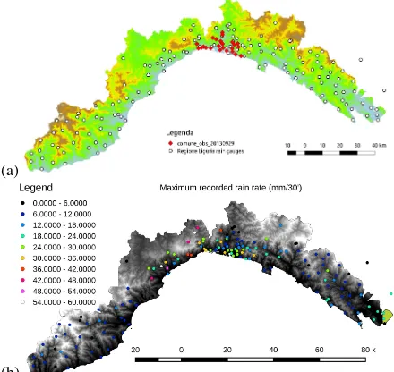
(a)
(b)
Figure 1: (a) Input rainfall measures at 143stations (regional level, white points) and25stations (municipality level, red cir-cles). (b) Map of the rain rate maximum recorded at each weather station, which highlights that only the central west of the region has been involved by heavy rain and the remaining part were in-terested by drizzle.
the underlying rainfall field. Indeed, they have a relevant seman-tic content and, at the same time, are formally well-defined. For this set of experiments, the approximated rainfalls were sampled at the vertices of a digital terrain model, producing a discretiza-tion of the precipitadiscretiza-tion field whose maxima were compared. The DTM used is coming from the SRTM (Shuttle Radar Topography Mission (Farr et al., 2007)), available in public domain at the URLhttp://www2.jpl.nasa.gov/srtm/, and with a spatial resolution of 100 mt.
4. THEORETICAL BACKGROUND
In the following, we give an overview of the three approxima-tion methods compared and of the persistence analysis frame-work used to analyze the evolution of precipitations (Fig. 2).
4.1 Approximation schemes
(a)
(b)
(c)
Figure 2: Rainfall fields computed for the event of September, 23: (a) LR B-Spline, (b) RBF, (c) Kriging.
be in the magnitude of(d1+ 1)×(d2+ 1)whered1andd2are
the polynomial degrees in the two parameter directions of the sur-face. The surface is bi-quadratic sod1=d2= 2. In our tests, the
algorithm is run with 20 iterations giving a total of3×20×N×9 bi-variate B-spline evaluations.
Implicit approximation with radial basis functions Implicit approximation computes the mapF(p) := Pni=1αiϕi(p)as
a linear combination of the basis B := {ϕi(p) := ϕ(kp− pik2)}ni=1, whereϕis the kernel function (Aronszajn, 1950, Dyn
et al., 1986, Micchelli, 1986, Patan`e et al., 2009). Depending on the properties ofϕ, we distinguish globally- (Carr et al., 2001, Turk and O’Brien, 2002) and compactly-supported (Wendland, 1995, Morse et al., 2001) supported radial basis functions. Then, the coefficients(αi)n
i=1 solve an×nlinear system, which is
achieve by imposing the interpolating constraintsF(pi) =f(pi), i = 1, . . . , n. Since an ×n linear system is solved once, the computational cost of the approximation with globally- and locally-supported RBFs isO(n3
)andO(nlogn), respectively. In our experiments, we have chosen the Gaussian kernelϕ(st) := exp(−st), which has a global support; in fact, its fast decay makes it suitable to approximate rainfalls with a sparse spatial distribution that change quickly in time. To this end, the width of each basis function is automatically adapted to the local sam-pling density by selecting its width according to the local spatial distribution of the rainfall stations (Dey and Sun, 2005, Mitra and Nguyen, 2003).
Kriging The previous two approximation methods do not take into account in an explicit manner; correlation among observa-tions may have unwanted effects especially in the case of un-evenly distributed observations. Furthermore, there is no natural mechanism for propagating the individual quality of the obser-vations into a quality description of the estimation. A class of methods that takes care of these issues is kriging, (Wackernagel, 2003), which is a common technique in environmental sciences and a special case of the maximum likelihood estimation. The underlying assumptions are that the quality of the observations
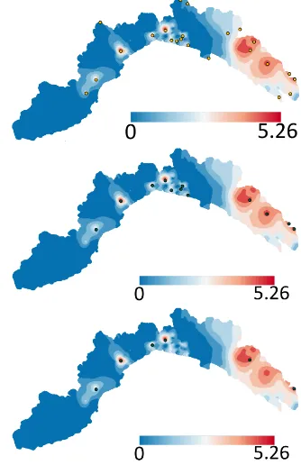
Figure 3: A function F : M → R, color-coded from blue (low) to red (high) values, and the associated local maxima hav-ing persistence greater thanα(maxF−minF), withα= 0.05, 0.15 (middle) and 0.25.
is given as variance values, and that the covariance between ob-servations only depends on their mutual spatial or temporal dis-tance, and not on their location. Formally, kriging is expressed asF(p) :=Pn
i=1ωif(pi), where the weightsωiare defined as
Ω = C−1
×DwithCthe covariance matrix of the measured values and Dis the matrix defined by the covariance between the known values and the points to be estimated. The covariance is expressed by the variogram model, which reflects the priors on the spatial variability of the values. The main problem with kriging is the low computational efficiency, as the solution of the linear systems scales quadratically with the number of observa-tions. In the implementation used, the problem is addressed by combining kriging with deterministic spatial division techniques, which efficiently restrict the number of observations to the clos-est ones. More specifically, theKd-tree is used to select only the 20 closest neighbors for the matrix inversion.
4.2 Prominent rainfall maximaviapersistence analysis
The importance of precipitation maxima is evaluated by means of thepersistence analysis. Given a scalar fieldF : M → R
(e.g., the interpolated rainfall field) and sweepingtin R, new connected components of the superlevel setsMt ={p∈ M: F(p)≥t}are either born, or previously existing ones are merged together. A connected component is associated with a local max-imum pof F, where the component is first born. When two components corresponding to local maximap1, p2, F(p1) < F(p2), merge together the component corresponding top1dies. In this case, the component associated with the smaller local max-imum is merged into that associated with the larger one. Each local maximumpofFis associated with its apersistence value persF(p), which is defined as the difference between the birth and the death level of the corresponding connected component. Maxima associated with a higher persistence value identify rele-vant features and structures of the underlying phenomena.
val-Method Max Mean Median Std. dev. MSE
Method [mm] [mm] [mm] [mm] [mm2]
Ord. krig. 32.44 (54.1%) 0.02 5.85E-05 2.38 5.64 RBFs 37.80 (63.0%) 0.97 0.34 2.12 5.44 LR B-Splines 27.2 (45.3%) -0.04 1.20E-5 2.73 7.05 Table 1: Summary statistics for the error distribution of the cross validation.
Figure 4: Leave-one-out cross validation MSE:y-axis reports the MSE [mm2
] for each time stepx-axis.
ues,Fis interpolated on the vertices of a triangle meshM. The points ofMare first sorted in decreasing values, frommaxFto minF; then, the classical 0th-persistence algorithm (Edelsbrun-ner et al., 2002, Edelsbrun(Edelsbrun-ner and Harer, 2010) is used. The cost of sorting thenpoints ofMisO(nlogn); by using a union-find data structure, the persistence algorithm requires linear storage and running time at most proportional toO(mα(m)), wherem is the number of edges in the mesh andα(·)is the inverse of the Ackermann function. An example for the extraction of local maxima at three different persistence levels is given in Fig. 3.
5. APPROXIMATION BEHAVIOR
The first set of results we discuss is related to the comparison of the behavior of the three methods according to approxima-tion performance and computaapproxima-tional complexity. Concerning the leave-one-out cross-validation strategy, we have checked the re-sults by computing the three approximation fields turning off, it-eratively, each rainfall station atpi, for each cumulated interval. The value of the approximation functionF obtained was then compared atpiwith the rain value measured by the correspond-ing rain gauge atpi, acting as a ground truth. The statistics of the evaluation are shown in Table 1; in this case, ordinary krig-ing and LR B-Splines have the smaller maximum error, but the RBFs have a smaller mean-squares error and standard devitation. In Fig. 4, the plot of the MSE distribution for the three methods is shown, per each time interval.
The second set of results concerns the cross-validation done using the rainfall data measured by the municipality stations as ground-truth to validate the values that approximate only the ARPAL data set. This validation aims at gathering indicators on the behavior, in terms of accuracy, on different spatial distribution of the sam-ple points. This approach is meaningful as the two observation networks cover an overlapping region of the study area. The net-work from Genova municipality is located within the boundary of the city and is denser than the ARPAL one, which covers the whole study area, and some of the ARPAL stations are located in the Genova municipality. Comparing the approximation re-sults at these two scales, we have evaluated the sensitivity of the approximation to local distributions of the samples and the capa-bility to estimate the local features of rain fields interpolated over
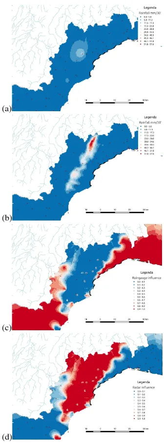
(a)
(b)
(c)
(d)
Figure 5: Ordinary kriging approximation of rainfalls computed with (a) rain gauges and (b) integrated with radar measurements. (c) Rain gauges weights and (d) radar data set mapped in (b).
a sparser data set. The results are shown in Table 2: in this case, ordinary kriging and LR B-Splines have the smaller maximum error, but the RBFs have a smaller mean-squares error.
Method Max Mean Median Std. dev. MSE
[mm] [mm] [mm] [mm] [mm2]
Ord. krig. 28.62 (47.7%) 0.59 3.26E-3 4.45 20.21 RBFs 36.77 (61.2%) 1.41 0.44 3.25 12.58 LR B-Splines 30.39 (50.6%) 0.59 3.71E-3 4.45 20.19 Table 2: Summary statistics for the error distribution of the accu-racy evaluation at different scales.
Table 3: Statistics for the average number of extracted persistent maxima.
Method τ=0.05 τ=0.15 τ=0.25 τ=0.35
Ord. krig. 7.4375 3.4792 2.3334 1.7292
RBFs 6.8750 3.4 2.4250 1.7250
LR B-Splines 7.6667 3.7917 2.5208 1.8333
obtained integrating radar rain data are presented.
6. PERSISTENT RAINFALL MAXIMA
Tables 3 and 4 report the comparative results about the extrac-tion of persistent maxima when considering the rainfall fields produced by the three approximation schema. For our tests, rain-fall fields have been computed based on the data set described in Sect. 3.. Hence, for each approximation scheme, we consid-ered the 48 approximated fields, one for each cumulative step. For each fieldF, the associated persistence maxima have been extracted according to four different values for the persistence thresholdε, namelyε = τ(maxF −minF) withτ = 0.05, 0.15, 0.25, 0.35. In practice, a maximum is preserved only if its persistence is larger than ε, while the others are filtered away. Table 3 reports the total number of extracted persistent maxima, averaged by the amount of considered cumulative steps; Table 4 shows the maximum number of local maxima that have been ex-tracted, method by method, from the 48 rainfall fields. Despite some slight differences in the results, the general trend is to have a decreasing number of persistent maxima as the thresholdτ in-creases. This is actually not surprising, since a higher persistence threshold implies that a larger portion of local maxima are pruned out. Also, for low values of the persistence threshold, we can relate the number of detected maxima to the smoothness of the considered approximation: in this view, the RBF schema appears to have a higher smoothing effect, as indicated by the smaller number of maxima characterized by a low persistence value.
6.1 Comparing sets of persistent maxima
In order to refine the above comparative analysis, we make use of the tracking procedure introduced in (Biasotti et al., 2015) to quantitatively assess a (dis)similarity measure between two sets of local maxima, originated from the three approximation schema when considering the same cumulative step. Before presenting results, we briefly recall the main ideas of (Biasotti et al., 2015).
For two setsF,Gof local maxima of two rainfall fieldsF, G :
M →R, it is possible to compare them by measuring the cost of moving the points associated with one function to those of the other one, with the requirement that the longest of the trans-portations should be as short as possible. Interpreting the local maxima inF andGas points inR3 (i.e., geographical position and persistence value), the collections of local maxima are com-pared through thebottleneck distancebetweenFandG, which is defined as
dB(F,G) = inf
γ supp d(p, γ(p)),
wherep∈ F,γranges over all the bijections betweenFandG, d(·,·)is thepseudo-distance
d(p,q) := min{kp−qk,max{persF(p),persG(q)}},
which measures the cost of movingptoq, andk · kis a weighted modification of the Euclidean distance. In practice, the cost of
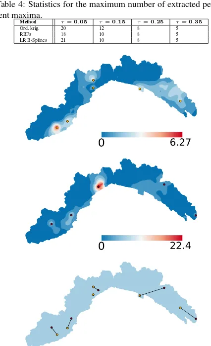
Table 4: Statistics for the maximum number of extracted persis-tent maxima.
Method τ=0.05 τ=0.15 τ=0.25 τ=0.35
Ord. krig. 20 12 8 5
RBFs 18 10 8 5
LR B-Splines 21 10 8 5
Figure 6: Two fieldsF, G : M → R, color-coded from blue (low) to red (high) values, and the associated local maxima. On the right, bottleneck matching between local maxima.
takingptoqis measured as the minimum between the cost of moving one point onto the other and the cost of moving both points onto the planexy : z = 0. Matching a pointpwith a point ofxy, which can be interpreted as the annihilation ofp, is allowed by the fact that the number of points forFandGis usu-ally different. The matchingγbetween the points ofFand those ofG, for whichdB is actually occurred, is referred to as a bot-tleneck matching(Fig. 6). Through the bottleneck matching and the bottleneck distance, it is then possible to derive quantitative information about the differences in the spatial arrangement and the rain measurements for the points inFandG.
The bottleneck distance can be evaluated by applying a pure graph-theoretic approach or by taking into account geometric infor-mation that characterize the assignment problem. We opt for a graph-theoretic approach, which is independent of any geometric constraint and our implementation is based on the push-relabel maximum flow algorithm (Cherkassky and Goldberg, 1997). For each iteration, the algorithm runs inO(k2.5
), wherekis the num-ber of local maxima involved in the comparison. We note that the computational complexity is not an issue, because the number of points to be considered is very limited in general. For example, in tracking applications the number of persistent maxima to be monitored is usually no more than a dozen for each time sample.
Table 5: Table of results for the averaged geographical distance (measured in km) between sets of local maxima (Liguria area size: 5.410 km2
).
Method1/Method2 τ=0.05 τ=0.15 τ=0.25 τ=0.35 Ord. krig / RBFs. 15.514 km 2.798 km 2.768 km 2.685 km RBFs / LR B Spline 35.08 km 10.30 km 5.71 km 4.054 km krig / LR B-Splines 35.36 km 6.528 km 3.388 km 2.326 km
Table 6: Table of results for the averaged rainfall distance (mea-sured in mm) between sets of local maxima.
Method1/Method2 τ=0.05 τ=0.15 τ=0.25 τ=0.35 Ord. krig/RBFs. 4.127 mm 2.438 mm 1.900 mm 1.884 mm RBFs/LR B Sp. 9.029 mm 5.111 mm 3.930 mm 3.960 mm Krig./LR B-Sp. 6.707 mm 3.345 mm 2.105 mm 1.991 mm
the sets of local maxima according to the four persistence thresh-olds discussed above. For each threshold, the three collections of persistent maxima are pairwise compared as follows. Since ge-ographic coordinates and rainfall measurements come with dif-ferent reference frames and at difdif-ferent scales, local maxima to be matched are first normalized so that their coordinates range in [0,1]; then, they are processed by computing the associated bottleneck matching and the bottleneck distance, and afterwards projected back in the original reference frames. Finally, a mea-sure of their distance in terms of both geographical coordinates and rainfall values is derived by combining the information con-tained in the bottleneck matching and the associated numerical (dis)similarity score. Precisely, we consider thegeographicaland rainfall distances, which are defined as the largest difference in geographical position and rainfall value, respectively, for two per-sistent maxima that have been paired by the bottleneck matching.
Tables 5 and 6 report the obtained results, in terms of geographi-cal and rainfall distances, respectively, averaged by the total num-ber of considered cumulative steps. To have a clearer picture of the comparative evaluation in terms of the two distances, the results included in Tables 5 and 6 should be jointly interpreted for each persistence threshold. For instance, when τ = 0.05 we have (relatively) high values for the geographical distance to-gether with quite low rainfall distance values: this can be inter-preted as slight numerical variations for the three approximations, possibly appearing spatially far one from each other. Note, how-ever, that in this view that the RBF and the kriging techniques appear to have a more similar behavior, both producing higher values for the geographical and rainfall distances when compared with LR-B Splines. On the other hand, moving to higher persis-tence thresholds, the values of geographical distance decrease, as an effect of filtering out non-relevant maxima. As a consequence, the corresponding rainfall distance values reveal now the differ-ences occurring at prominent maxima, which appear to be quite small.
We conclude by proposing in Table 7 a similar analysis to com-pare the results that are obtained when rainfall fields are inter-polated by considering either observed rainfall measurements or an integration of these data with radar acquisitions (Sect. 5.). In-deed, integrated data can reveal useful, e.g., for tracking appli-cations: although rainfall measurements are more reliable, inte-grating them with radar data makes it possible to extend the rain-fall field interpolation in larger areas and to have a clearer picture about the temporal evolution of the associated precipitation event. As can be seen from the results in Table 7, characterized by high values in both the geographic and the rainfall distance, consid-ering radar data can sensibly change the spatial location and the rainfall value of persistent maxima. This can be interpreted as the introduction of complementary information with respect to rain-fall measurements, which hopefully can help in having a clearer understanding of precipitation events.
Table 7: Averaged geographical (measured in km) and rainfall distance (measured in mm) between sets of local maxima.
Krig/(Radar + Krig) τ=0.05 τ=0.15 τ=0.25 τ=0.35 Geogr. dist. 45.453 km 23.387 km 18.568 km 13.28 km Rainfall dist. 23.97 mm 21.227 mm 18.533 mm 16.396 mm
7. CONCLUSIONS AND FUTURE WORK
The aim of this study was the comparison of different spatial ap-proximation methods finalized to compute the amount of rainfalls for hydro-metereological analysis and civil protection. As a final remark, we point out that all these approaches easily support the integration of further sources of rain measures, for instance those captured by radar. Fig. 5 shows the results of estimation achieved by kriging (a) with the rain gauges only and (b) with the inte-gration of this data with radar information. In (c,d), we show the contribution of each data set in the estimated map plotted in (b). The color scale varies from blue to red corresponding respec-tively to a contribution varying from null to full. Since we have selected only two different data sets, the two maps in (c,d) are complementary.
Finally, we plan to proceed further with the presented compari-son framework, including several more aspects and extending the evaluation to more elaborate correlation analysis, taking into ac-count other relevant data, such as terrain morphology, satellite imagery, and meteorological situation. We will further investi-gate this possibility and especially the effect on approximation results on storm tracking.
Acknowledgments This work has been supported by the FP7 Integrated Project IQmulus, FP7-ICT-2011-318787. The rainfall data sets are courtesy of ARPAL, Regione Liguria, and of the Genova Municipality.
REFERENCES
Aronszajn, N., 1950. Theory of reproducing kernels. Trans. of the American Mathematical Society 68, pp. 337–404.
Azimi-Zonooz, A., Krajewski, W., Bowles, D. and Seo, D., 1989. Spatial rainfall estimation by linear and non-linear co-kriging of radar-rainfall and raingage data. Stochastic Hydrology and Hy-draulics 3(1), pp. 51–67.
Biasotti, S., Cerri, A., Pittaluga, S., Sobrero, D. and Spagnuolo, M., 2015. Persistence-based tracking of rainfall field maxima. Topology-Based Methods in Visualization 2015, In press.
Brocca, L., Ciabatta, L., Massari, C., Moramarco, T., Hahn, S., Hasenauer, S., Kidd, R., Dorigo, W., Wagner, W. and Levizzani, V., 2014. Soil as a natural rain gauge: Estimating global rain-fall from satellite soil moisture data. Journal of Geophysical Re-search: Atmospheres 119(9), pp. 5128–5141.
Carr, J. C., Beatson, R. K., Cherrie, J. B., Mitchell, T. J., Fright, W. R., McCallum, B. C. and Evans, T. R., 2001. Reconstruction and representation of 3D objects with radial basis functions. In: ACM Siggraph, pp. 67–76.
Cherkassky, B. V. and Goldberg, A. V., 1997. On Implement-ing the Push-Relabel Method for the Maximum Flow Problem. Algorithmica 19(4), pp. 390–410.
Dey, T. K. and Sun, J., 2005. An adaptive MLS surface for re-construction with guarantees. In: ACM Symposium on Geometry Processing, pp. 43–52.
Di Piazza, A., Conti, F., Noto, L., Viola, F. and La Loggia, G., 2011. Comparative analysis of different techniques for spa-tial interpolation of rainfall data to create a serially complete monthly time series of precipitation for sicily, italy. International Journal of Applied Earth Observation and Geoinformation 13(3), pp. 396–408.
Dixon, M. and Wiener, G., 1993. Titan: Thunderstorm identifica-tion, tracking, analysis, and nowcasting–a radar-based method-ology. Journal of Atmospheric and Oceanic Technology 10(6), pp. 785–797.
Dokken, T., Lyche, T. and Pettersen, K. F., 2013. Polynomial splines over locally refined box-partitions. Computer Aided Ge-ometric Design 30(3), pp. 331–356.
Dyn, N., Levin, D. and Rippa, S., 1986. Numerical procedures for surface fitting of scattered data by radial functions. SIAM Journal on Scientific and Statistical Computing 7(2), pp. 639–659.
Edelsbrunner, H. and Harer, J., 2010. Computational Topology: An Introduction. American Mathematical Society.
Edelsbrunner, H., Letscher, D. and Zomorodian, A., 2002. Topo-logical persistence and simplification. Discrete Computational Geometry 28, pp. 511–533.
Farr, T. G., Rosen, P. A., Caro, E., Crippen, R., Duren, R., Hens-ley, S., Kobrick, M., Paller, M., Rodriguez, E. and Roth, L., 2007. The shuttle radar topography mission. Reviews of Geophysics 45(2), pp. 361–363.
Goovaerts, P., 1997. Geostatistics for natural resources evalua-tion. Oxford University Press.
Goovaerts, P., 2000. Geostatistical approaches for incorporating elevation into the spatial interpolation of rainfall. Journal of Hy-drology 228(1), pp. 113–129.
Han, L., Fu, S., Zhao, L., Zheng, Y., Wang, H. and Lin, Y., 2009. 3D Convective Storm Identification, Tracking, and Forecasting– An Enhanced TITAN Algorithm. Journal of Atmospheric and Oceanic Technology 26(4), pp. 719–732.
Hong, Y., Adler, R. and Huffman, G., 2007. An experimental global prediction system for rainfall-triggered landslides using satellite remote sensing and geospatial datasets. IEEE Trans. on Geoscience and Remote Sensing 45(6), pp. 1671–1680.
Hou, A. Y., Ramesh, K. K., Neeck, S., Azarbarzin, A. A., Kum-merow, C. D., Kojima, M., Oki, R., Nakamura, K. and Iguchi, T., 2014. The global precipitation measurement mission. Bulletin of the American Meteorological Society.
Johnson, J. T., MacKeen, P. L., Witt, A., Mitchell, Stumpf, G. J., Eilts, M. D. and Thomas, K. W., 1998. The Storm Cell Identifi-cation and Tracking Algorithm: An Enhanced WSR-88D Algo-rithm. Wea. Forecasting 13(2), pp. 263–276.
Journel, A. G. and Huijbregts, C. J., 1978. Mining geostatistics. Academic press.
Keefer, D., Wilson, R., Mark, R., Brabb, E., Brown, W., Ellen, S., Harp, E., Wieczorek, G., Alger, C. and Zatkin, R., 1987. Real-time landslide warning during heavy rainfall. Science 238, pp. 921–925.
Kucera, P. A., Ebert, E. E., Turk, F. J., Levizzani, V., Kirschbaum, D., Tapiador, F. J., Loew, A. and Borsche, M., 2013. Precipita-tion from space: advancing earth system science. Bulletin of the American Meteorological Society 94, pp. 365–375.
Lakshmanan, V. and Smith, T., 2009. An Objective Method of Evaluating and Devising Storm-Tracking Algorithms. Wea. Fore-casting 25(2), pp. 701–709.
Lee, S., Wolberg, G. and Shin, S. Y., 1997. Scattered data inter-polation with multilevel b-splines. IEEE Trans. on Visualization and Computer Graphics 3(3), pp. 228–244.
McCuen, R. H., 1989. Hydrologic analysis and design. Prentice-Hall Englewood Cliffs, NJ.
McRobie, F. H., Wang, L.-P., Onof, C. and Kenney, S., 2013. A spatial-temporal rainfall generator for urban drainage design. Water Science and Technologies 68(1), pp. 240–249.
Micchelli, C. A., 1986. Interpolation of scattered data: Distance matrices and conditionally positive definite functions. Construc-tive Approximation 2, pp. 11–22.
Mitra, N. J. and Nguyen, A., 2003. Estimating surface normals in noisy point cloud data. In: Proc. of Computational Geometry, ACM Press, pp. 322–328.
Morse, B. S., Yoo, T. S., Chen, D. T., Rheingans, P. and Subrama-nian, K. R., 2001. Interpolating implicit surfaces from scattered surface data using compactly supported radial basis functions. In: IEEE Shape Modeling and Applications, pp. 89–98.
Patan`e, G., Spagnuolo, M. and Falcidieno, B., 2009. Topology-and error-driven extension of scalar functions from surfaces to volumes. ACM Trans. on Graphics 29(1), pp. 1–20.
Scheuerer, M., Schaback, R. and Schlather, M., 2013. Interpo-lation of spatial data - a stochastic or a deterministic approach? European Journal of Applied Mathematics 24, pp. 601–629.
Segond, M.-L., 2007. The significance of spatial rainfall rep-resentation for flood runoff estimation: A numerical evaluation based on the Lee catchment. Journal of Hydrology 347, pp. 116 – 131.
Skok, G. and Vrhovec, T., 2006. Considerations for interpolat-ing rain gauge precipitation onto a regular grid. Meteorologische Zeitschrift 15(5), pp. 545–550.
Teegavarapu, R. S. V. and Chandramouli, V., 2005. Im-proved weighting methods, deterministic and stochastic data-driven models for estimation of missing precipitation records. Journal of Hydrology 312(1), pp. 191–206.
Thiessen, A. H., 1911. Precipitation averages for large areas. Monthly weather review 39(7), pp. 1082–1089.
Turk, G. and O’Brien, J. F., 2002. Modelling with implicit sur-faces that interpolate. ACM Siggraph 21(4), pp. 855–873.
Wackernagel, H., 2003. Multivariate geostatistics: an introduc-tion with applicaintroduc-tions. 2nd edn, Springer-Verlag.
Wake, B., 2013. Flooding costs. Nature Climate Change 3(9), pp. 1671–1680.
Wendland, H., 1995. Real piecewise polynomial, positive defi-nite and compactly supported radial functions of minimal degree. Advances in Computational Mathematics 4(4), pp. 389–396.