www.elsevier.nlrlocaterjappgeo
Mathematical models and controlled experimental studies
Three-dimensional inversion of induced polarization data from
simulated waste
1A. Weller
a,), W. Frangos
b, M. Seichter
ca
Institut fur Geophysik, Technische Uni¨ Õersitat Clausthal, Arnold-Sommerfeld-Str. 1,¨
D 38678 Clausthal-Zellerfeld, Germany
b
Earth Science DiÕision, Lawrence Berkeley National Lab, 1 Cyclotron Road, Berkeley, CA 94720, USA
c
Institut fur Geophysik und Meteorologie, Technische Uni¨ Õersitat Braunschweig, Mendelssohnstr. 3,¨
D 38106 Braunschweig, Germany
Received 25 March 1998; accepted 13 November 1998
Abstract
Ž . Ž .
The Idaho National Laboratory INEL Cold Test Pit CTP has been carefully constructed to simulate buried hazardous
Ž .
waste sites. An induced polarization IP survey of the CTP shows a very strong polarization and a modest resistivity
Ž .
response associated with the simulated waste. A three-dimensional 3-D inversion algorithm based on the simultaneous
Ž .
iterative reconstruction technique SIRT and finite difference forward modelling has been applied to generate a subsurface model of complex resistivity. The lateral extents of the waste zone are well resolved. Limited depth extent is recognized, but the bottom of the waste appears too deep. With a modelling experiment, the intrinsic polarizability of the waste material is determined. Since IP is a technique for detection of diffuse occurrences of metallic material, this method holds promise as a method to distinguish buried waste from conductive soil material.q2000 Elsevier Science B.V. All rights reserved.
Keywords: Electrical resistivity; Geoelectrical prospection; Induced polarization; Inversion algorithm
1. Introduction
A variety of radioactive and hazardous waste material has been disposed of over the years at the Idaho National Engineering Laboratory
ŽINEL . Precise location is unknown for some.
)Corresponding author. Tel.:
q49-5323-722233; Fax: q49-5323-722320; E-mail: [email protected]
1
This paper was also published in Journal of Applied
Ž .
Geophysics, Vol. 41 1999 31–47. PII no. of original
Ž .
article: PII: S0926-9851 98 00036-6.
of the waste dumps. In order to test various methods of non-invasive subsurface waste loca-tion techniques, a simulated waste pit has been constructed using safe materials, and designed to resemble old waste pits as closely as possible
Že.g., size, depth, order and disorder of contents,
.
allowance for deterioration of containers . This
Ž .
Cold Test Pit CTP has been investigated by a number of workers using several different meth-ods. The present work was carried out as part of the Electromagnetic Integrated Demonstration
ŽEMID , which also includes an assortment of. Ž
electromagnetic techniques VETEM, 1996;
.
Pellerin and Alumbaugh, 1997 .
0926-9851r00r$ - see front matterq2000 Elsevier Science B.V. All rights reserved.
Ž .
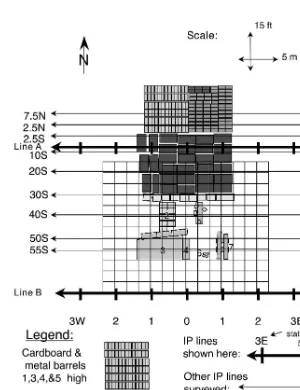
The CTP was constructed as a 13=70 m trench, segmented by transverse berms into cells. The southernmost cell investigated in the EMID
Ž .
project Fig. 1 contains stacked drums and boxes and a variety of randomly positioned barrels, pipes, a large metal tank, etc. This location is referred to as the Large Object Pit
ŽLOP . The buried drums located in the centre.
of the trench include both cardboard and metal
Ž
drums containing scrap metal both ferrous and
.
non-ferrous and non-metallic materials. The
cardboard drums and wooden boxes have metal-lic rims. The cell is described as being a 3-m waste seam with about 1.5 m of soil cap, thus the depth of the bottom of the waste is about 4.5 m. The cap is composed of clay-rich soil im-ported from other areas of the INEL complex. Host material is local soil overlying resistive Snake River basalt.
The EMID project focused mostly on rapid electromagnetic techniques, which rely upon variations of conductivity. In contrast, the slower
Ž . Ž . Ž . Ž . Ž .
Fig. 1. Survey layout at the INEL CTP. 1 Boxes, 2 drum stack, 3 crushed drums, 4 steel tank, 5 concrete filled steel
Ž . Ž .
Žand therefore more expensive induced polar-. Ž .
ization IP method exploits electrochemical phenomena at interfaces between regions of metallic and electrolytic conduction within a heterogeneous medium.
While the first reported recognition of what
Ž .
we now call IP was by Schlumberger 1920 , much of its early development sprang from mine warfare research during World War II
ŽGrow, 1982; Collett, 1990 . The principal ap-.
plication of IP has been prospecting for dissemi-nated base and precious metal ore deposits, a technology transfer of the wartime research
ŽBleil, 1953; Collett, 1990 . In an early investi-.
gation of cultural contamination of domestic
Ž .
water supplies, Angoran et al. 1974 used IP to trace town dumps in the state of Massachusetts,
Ž .
USA. Frangos and Andrezal 1994 reported IP measurements over a landfill and toxic waste pond in Slovakia. The increase in resolution of small polarization effects in sediments enabled the successful application of IP measurements in environmental investigations such as the de-tection of contaminants or the determination of
Ž
hydraulic properties Vanhala et al., 1992;
.
Weller and Borner, 1996 .
¨
2. Induced polarization and complex conduc-tivity
The IP phenomena are of electrochemical origin and are caused either by metallic mineral particles in a rather poorly conducting rock matrix or by differences in the ion concentra-tions in the pore space or at the interface
be-Ž .
tween matrix and pore space Sumner, 1976 . Any current in a polarizable medium is hindered from flowing by the chargeability m of the
Ž .
medium Seigel, 1959 . Therefore, the conduc-tivity of a polarizable medium s0 is reduced with respect to the conductivity s of that medium without polarizable constituents
s0ss
Ž
1ym ..
Ž .
1The current flowing in one direction ‘charges’ all the polarizable elements, and generates a secondary voltage V . After a long duration ofs current flow all the elements are saturated, and the primary voltage V is reached. The values ofp
primary and secondary voltages may be approx-imated in time domain IP surveys performing
Ž .
voltage measurements immediately before Vp
Ž .
or after the feeding current is shut off V . Thes
chargeability is given by the ratio
Vs
ms .
Ž .
2Vp
A comparable quantity is determined in the frequency domain. In general, the amplitude of
< Ž .<
resistivity r v decreases with increasing fre-quency. If the resistivity is measured at two frequencies, with v1-v2, the frequency effect
ŽFE is calculated, thus:.
<r v
Ž
1.
<y<r vŽ
2.
<FEs < < ,
Ž .
3r v
Ž
2.
describing the fractional decrease of the resistiv-ity amplitude with increasing frequency.
Regarding a theoretical limit of the frequency effect, the apparent resistivity of the lower fre-quency v1 is estimated by the DC-value
Vp
r v
Ž
s0.
s K ,Ž .
4I
with I being the current, and K the geometric factor. The apparent resistivity at the higher frequencyv2 may be approximated by the limit
VpyVs
lim r v
Ž .
s K .Ž .
5v™` I
Using these limits, the results from measure-ments in time- and frequency-domain become transferable to each other:
m
FEs .
Ž .
6 1ymtime-domain measurements over a wide time-in-terval or spectral IP measurements recording the amplitude and phase angle in a frequency range. The resulting amplitude and phase spectra show the frequency dispersion of the apparent con-ductivity.
The electrical conductivitys of rocks, which includes both conduction and polarization ef-fects, generally may be presented as a complex
Ž X
.
quantity. Both the real s and the imaginary
Ž Y.
s parts are frequency dependent:
s v
Ž .
ssXŽ .
v qisYŽ .
v ,Ž .
7with v being the angular frequency and i the imaginary unit. The in-phase component corre-sponds to the intrinsic or Ohmic conductivity, and the quadrature component to polarization effects which are caused by a kind of capacitive conductivity component in rocks. A complex quantity can also be represented by the ampli-tude
2 2
X Y
<s v
Ž .
<s(
Ž
s vŽ .
.
qŽ
sŽ .
v.
,Ž .
8and the phase angle
sY
Ž .
vw v
Ž .
sarctanž
X/
.Ž .
9s v
Ž .
The reported phase angle is the phase shift between the injected current and the measured voltage caused by polarization effects. Note that if alternating current is used, the measured sig-nal is also influenced by induction effects which results in an additional phase shift. Complicated procedures to remove electromagnetic coupling
Ž .
from IP data Pelton et al., 1978 can be avoided if a frequency range and a geometry of voltage and current electrodes are used such that these effects can be ignored. Since the complex resis-tivityr is the inverse of the complex conductiv-itys
1
r v
Ž .
s ,Ž .
10s v
Ž .
a measurement of conductivity or resistivity can be transformed into each other. The sign of all
phase angles given below is related to the
defi-Ž .
nition in Eq. 9 .
An IP measurement run at a single frequency yields both resistivity amplitude and phase shift. The processing and interpretation of these mea-surements requires accurate and fast modelling and inversion algorithms. While geologic struc-tures like horizontally stratified media can be described by one-dimensional models, arbitrar-ily shaped bodies require two-dimensional or
Ž .
three-dimensional 3-D modelling and
inver-Ž
sion. In the IP frequency range i.e., below 10
.
Hz and survey geometry used herein, electro-magnetic effects are negligible.
Ž .
According to Eq. 1 , the ultimate effect of chargeability alters the effective conductivity of the media when current is applied. Thus, IP modelling can be performed by carrying out two forward DC modelling steps using the original conductivitys and a perturbed distribution s0. The apparent chargeability is obtained from these two DC results. This procedure is used in
Ž
many IP forward modelling programs e.g.,
.
Weller, 1986; Oldenburg and Li, 1994 .
In this paper, an alternative technique is used which is based on the originally measured quan-tities in the frequency domain. The IP equip-ment directly records the amplitude of the ap-parent resistivity and the phase shift between the injected current signal and the measured voltage. These two quantities describe a com-plex number, in this case a comcom-plex apparent resistivity, which is directly used in the inver-sion algorithm.
3. Experimental procedure
polariza-tion effects. We used porous pots approximately 4.5 cm in diameter with copper rods immersed in a saturated solution of copper sulfate. Electri-cal potential differences between pairs of these electrodes in a water bath were typically less than 2 mV. The pots were wetted, when
neces-Ž .
sary, with a small amount about 50 ml of tap
Ž
water to ensure low contact resistance typically
.
less than 2000 V without altering the near surface resistivity on this small scale.
Transmit-Ž
ter electrodes were single nails typically 5 cm
.
long wetted with 50–75 ml of salt water. Posi-tions of all electrodes were determined with a measuring tape, and location accuracy is typi-cally 5 cm.
A dipole–dipole array was chosen for the work at the CTP because it provides both profil-ing and soundprofil-ing information simultaneously. While other arrays may offer improved resolu-tion under some circumstances, the dipole–di-pole array is both economical and effective in a wide variety of conditions, and the electromag-netic coupling effects are smaller than in sym-metrical configurations. Fig. 1 shows the loca-tions of the eleven lines surveyed. Two elec-trode spacings were employed; all lines were measured with a 5-m spacing, while the north-ern four lines were also surveyed with a 2-m spacing. The 5-m lines provide more economi-cal coverage of the area and a better resolution of the bottom of the waste seam, while the 2-m data yield better resolution of the depth to waste. Please note that the INEL CTP survey grid is in feet, with its origin at the southwest corner of the stacked drums, while the IP survey is mea-sured in meters, with distances meamea-sured east and west of the centre line through the CTP. All line numbers follow the official grid, e.g., Line 20 S is 20 ft south of the drum stack. Station numbers are in dipole units from the transmitter position, e.g., station 3E is three dipoles east of the centre of the line, which is 15 m for 5-m spaced lines.
All data were acquired with two or three dual-channel Aquila model A-1 phase
measur-Ž .
ing IP receivers a multi-channel system
simi-Ž .
lar to that described by Frangos 1990 and a battery-powered, current-regulated transmitter.
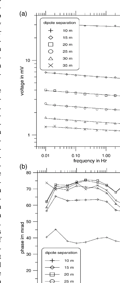
Voltage and phase spectra were observed on Line 7.5 N using 5-m dipoles between
frequen-Fig. 2. Spectra of complex resistivity measurements at Line 7.5 N, 5-m dipoles, transmitter at 0–1E, receivers to
Ž . Ž .
cies of 0.01 and 10 Hz. Transmitter dipole 0–1E was the source, and receivers were placed on six dipoles to the west. The amplitude
spec-Ž .
tra Fig. 2a show a considerable decrease with rising frequency which would result in strong frequency effects for all dipole separations. The slope can be well approximated by a straight line in double-logarithmic scale. The phase
Ž .
spectra Fig. 2b show large phase shifts which are virtually independent of frequency over the observed range and consistent with the mono-tonic decrease of amplitude with increasing
fre-quency. This behaviour corresponds to the
con-Ž
stant phase angle model van Voorhis et al.,
.
1973; Borner et al., 1991 .
¨
A single frequency was chosen for conve-nience in rapid data acquisition with the particu-lar instrumentation employed. The spectral tests showed that 1 Hz is representative of the IP response in this area.
The data are plotted in the standard
pseudo-Ž .
section format e.g., Sumner, 1976, pp. 43–46 , with resistivity reported in V m and IP as phase
Ž .
lag in milliradians mrad . Accuracy of the
sistivity data is principally limited by uncer-tainty of electrode locations and the transmitter current and appears to be generally within 5%. IP repeatability is approximately 2 mrad, based on numerous reciprocal repeat points in the survey.
4. Survey results
Ž .
Five-meter dipole data from Lines A 7.5 S
Ž .
and B 75 S are presented as Figs. 3 and 4,
respectively. The former are representative of results over the simulated waste, while the latter are as far removed from the waste as could be managed within the CTP. The results of Line B
ŽFig. 4 serve to illustrate the background resis-.
tivity and IP patterns over the CTP.
Clearly there is a huge IP response from the
Ž
simulated waste typical mining exploration
ap-.
parent IP responses are 20 to 50 mrad . Note that the ‘pants–leg’ pattern in Fig. 3, i.e., the two strong anomalous diagonals, is an artifact of the dipole–dipole pseudosection plotting
vention showing the apparent resistivity or phase lag in the centre of both dipoles. Regarding the real location of the dipoles, it becomes clear that the responses originate within a single re-gion near the middle of the line where one of the dipoles is placed. The negative apparent IP effects measured on Line A are due to body polarization effects, common in high-contrast circumstances involving 2- and 3-D bodies.
Relatively small IP effects are observed on the background line. Other measurements in the area suggest that the intrinsic polarization effect of the clay, soil, and basalt is less than 5 mrad, or somewhat less than the largest values ob-served on line B. Some residual IP effect is due to lateral effects from the ‘large objects’ only one dipole length to the north of the line.
The resistivity data of Fig. 3 show a conduc-tive zone located near the centre of the line, with apparent resistivities decreased to about one half to one third of background. This fea-ture forms a viable target for methods based on conductivity contrasts. Another prominent con-ductive feature on the eastern end of the
back-Ž .
ground line Fig. 4 is not due to any known waste and has no corresponding IP response. This non-waste-related resistivity response shows an apparent resistivity far less than that of the simulated waste, and appears on the short separations, indicating a shallow causative body. The feature was detected on some of the other lines as well as by several of the other survey methods used in the EMID work. The unknown conductive feature may be due to variations in the source, handling, or compaction of the cap material, or to subsequent modifications such as spills during operations in the area. In any case, it is clear that buried waste is not the only cause of conductive anomalies at INEL.
5. Forward modelling and inversion
The structures at a waste dump require gener-ally a 3-D data interpretation. The software for
data processing includes forward modelling and inversion procedures. The algorithm used for forward modelling considers both conductivity
s and potential V as complex quantities. The forward modelling algorithm proposed by
Ž .
Weller et al. 1996a is summarized as follows. For a current I fed at a point A represented by the vector r , the resulting electrical poten-A
Ž < .
tial V r rA satisfies the equation of continuity
<
=P s
Ž .
r =V r rŽ
A.
qIdŽ
ryrA.
s0,Ž .
11where d is the Dirac delta function. This equa-tion is solved in a discrete space of two or three
Ž .
dimensions by the finite difference FD method. In usual modelling geometries, the upper boundary of the model is given by the earth’s surface, where Neumann boundary conditions are satisfied. For all other boundaries of the model which are drawn inside the conducting medium, mixed boundary conditions as
pro-Ž .
posed by Dey and Morrison 1979 are applied. The grid may be presented as an electrical network.
The resulting system of equations is written in matrix form, where each equation corre-sponds to Kirchhoff’s Current Law for a single node. The complex matrix of coupling coeffi-cients is symmetric but not Hermitian. A com-pact storage scheme fully uses the sparcity and symmetry of the matrix while a generalized conjugate gradient method solves the system of equations. Preconditioning techniques speed up the solution.
The forward problem is solved for each cur-rent source separately. The appacur-rent complex resistivities for all configurations can be com-puted easily by a superposition of several pole–pole configurations. In the case of multi-electrode-arrays, this method reduces the num-ber of forward problems to the numnum-ber of cur-rent electrode positions. The number of mea-sured configurations is generally much higher.
value is influenced by both the conductivity distribution in a large volume of earth and the electrode configuration, a pseudosection can only be a distorted reflection of the real subsur-face structures. The reconstruction of the con-ductivity distribution is performed by inversion techniques. Incorporating all available
informa-Ž
tion into the inversion process Olayinka and
.
Weller, 1997 can reduce the non-uniqueness inherent in 2-D and 3-D interpretation.
The objective of inversion consists of finding a conductivity model which can approximate the measured data within the limits of data errors and which is in agreement with all a priori information. The inversion can be done manually by forward modelling in which changes in the model parameters are made by trial and error until a sufficient agreement be-tween measured and synthetic data is achieved. For more complicated structures, where the number of parameters increases, automatic in-version procedures are recommended.
The inversion algorithm used is applicable to variable electrode configurations including buried electrodes. It is based on a simultaneous
Ž .
iterative reconstruction technique SIRT , which has been applied to several tomographic
prob-Ž
lems to solve systems of linear equations e.g., Dines and Lytle, 1979; van der Sluis and van
.
der Vorst, 1987 . It can be used for both 2-D and 3-D inversion. Since the number of grid elements is generally much higher than the number of measured data, a strongly underde-termined system has to be solved.
The steps involved in the iterative procedure are as follows.
Ž .a The subsurface is subdivided into blocks of constant resistivity. The number of blocks N is equal to the number of model parameters. All parameters may be described by a parameter
Ž .T
vector xs x , . . . , x1 N . The parameter xj is defined as the logarithm of the resistivity of the jth block.
Ž .b The measured data are compiled in a data
Ž .T
vector y
ˆ
s y , . . . , yˆ
1ˆ
M where M corresponds to the number of measurements. The element yˆ
iof the data vector y is the logarithm of the
ˆ
complex apparent resistivity of the ith measure-ment in the data set. The use of the logarithms of resistivities instead of resistivities has proven to be more appropriate in inversion because negative resistivities are avoided and relative changes are emphasized.
Ž .c A starting model is chosen. The parameter vector is initialized xsxŽ0..
Ž .d The forward modelling for the model xŽk.
is performed where k denotes the number of the model. The apparent resistivity is calculated for all M configurations of electrodes used in the survey. The calculated data are compiled in a data vector yŽk.. The forward modelling is
de-scribed by an operator S which is applied to the parameter vector xŽk.:
yŽk.
sS x
Ž
Žk..
.Ž .
12Although the forward modelling operator S is nonlinear, an attempt was made to use SIRT for
Ž .
a linearization of Eq. 12 in the vicinity of the model xŽk.
Ž .
Žk. k
ysy qS x
Ž
yx.
.Ž .
13The matrix S is the Jacobian or sensitivity ma-trix
called sensitivities describing the influence of a slight change of the resistivity of a single grid element on the measured apparent resistivity of a given configuration. The forward modelling is performed by the finite difference method.
Ž .e The residual rŽk. between measured and
computed data is determined:
rŽk.sy
ˆ
yyŽk..Ž .
165 Žk.5
the data accuracy the iteration process is stopped. The last model is accepted as a solution of the inversion.
Ž .f If the residual fails the stopping criterion, the differences are applied to correct the resis-tivity model according to the general equation
1 si , j
inversion algorithm, Eq. 17 is used with an exponent as1 which has been proven to be a good choice concerning the rate of convergence. A relaxation factor 1.2-v-1.7 should be used to speed up the procedure.
The next iteration is started with the forward
Ž .
modelling in step d .
If no starting model is prescribed, one would be generated by a back projection according to the formula
using only positive sensitivities for a homoge-neous subsurface resistivity distribution. The back projection which may be called an approx-imate inversion yields a model showing the main features of the subsurface at low contrasts.
Ž .
The iterative application of Eq. 17 describes the procedure of a generalized matrix inversion without explicitly calculating the inverse matrix. Without any smoothness constraint, the SIRT generates models with low contrasts in the de-termined parameters. The duplicate weighing by the sums of the absolute values of sensitivities
Ž .
inherent in Eq. 17 is responsible for a stable convergence and the resulting smooth models.
An efficient application of SIRT requires a fast and accurate algorithm to calculate the sen-sitivity matrix S. Since the logarithms of both the model resistivity rj and the apparent
resis-Ž .
In the case of a homogeneous resistivity dis-tribution with all model resistivities rjsrhs
const, the resulting apparent resistivity becomes constant r
ˆ
jsrh, and the sensitivities si, j and s˜
i, j are equal.Following an algorithm described by Weller
Ž .
et al. 1996b and using the abbreviation
< < 3
s
ˆ
A, MsH
=V r rŽ
A.
=V r rŽ
M.
d r ,Ž .
21Vj
the sensitivity of any four point configuration with the corresponding geometric factor K re-i
sults in potentials for a current source at the locations A and M, respectively. The sensitivity calculation for a given pole–pole configuration with the current electrode A and the potential electrode M demands two separate forward runs with the source subsequently located at the transmitter position A and the receiver position M. The decomposition of all configurations in the basic pole–pole readings has proven to be advanta-geous for the application of multi-electrode-arrays, because the number of measured config-urations is generally much higher than the num-ber of electrodes.
halfspace and all electrodes on the surface Eq.
Ž21 results in the expression.
I2r2 1 1
j 3
s
ˆ
A, Ms 2H
=< <=< <d r ,Ž .
23V
4p j ryrA ryrM
which can be easily calculated.
Since a change in the model results in a change of the sensitivities, these have to be updated. Tests have shown that an update of the sensitivity matrix in each iteration results only in a slight improvement of the rate of conver-gence compared with the use of unchanged halfspace sensitivities. Since the computational effort of a sensitivity update is considerable, current experience suggests that it should be performed only after every five or ten iterations.
6. Inversion results
The IP survey at the CTP was not originally planned for interpretation by a 3-D inversion algorithm. All the measurements were made on east–west trending profiles that were not equally spaced. The distances between the neighbouring profiles vary between 0.76 and 6.1 m. An opti-mal 3-D survey should be performed on an equally spaced grid with profiles in perpendicu-lar directions.
The large amount of IP data acquired in a relatively small area over structures which can-not be regarded as two-dimensional suggested a test of a 3-D inversion algorithm that was devel-oped to monitor hydraulic experiments with cross-hole measurements of complex
conductiv-Ž .
ity in isolated tanks Weller et al., 1996b . The inversion of the data set from the CTP was the first test with IP field data.
A first grid was generated for the inversion of all the data acquired with 5-m dipole spacing
Ždata set 1 . The resulting grid consists of 27,984. Ž
nodes with 53 steps in the x-direction west–
. Ž .
east , 33 in the y-direction south–north , and
Ž .
16 in the z-direction depth . Data set 1 includes 638 measurements from all the eleven lines.
Average values are used for the reciprocal re-peat points. The back projection resulted in a
Ž .
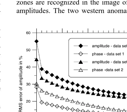
model with a root mean square RMS error of 55.0% in the amplitude and 28.2 mrad in the phase angle compared with the measured val-ues. After 20 steps of iteration performed on a Pentium Pro 200 microcomputer in 21,437 s, the RMS error has fallen to 22.8% in the ampli-tude and 11.3 mrad in the phase. The continu-ous decrease of the errors during the iteration process is presented in Fig. 5. The sensitivity matrix has been updated after the second and eighth step of iteration. During the first steps, a rapid decrease in error is observed. The last steps result only in slight improvement of the model. The covergence rate slows down. Since the residual did not reach the estimated data accuracy the maximum number of iterations was performed.
The inversion results in a 3-D data matrix with each component describing the amplitude and phase value of a resistivity grid element. Horizontal and vertical planes of data are ex-tracted from this 3-D matrix.
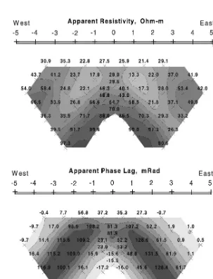
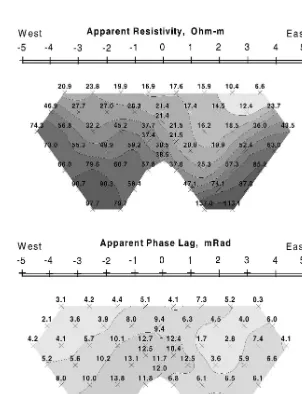
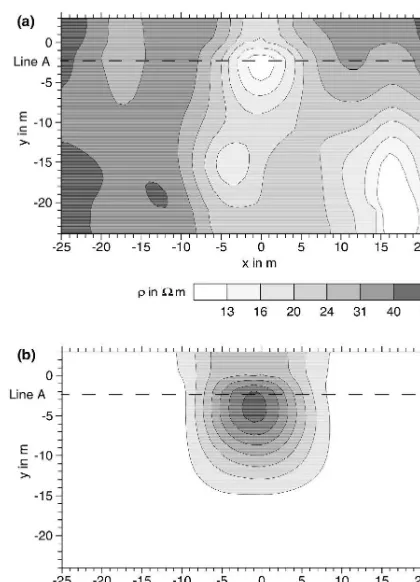
The horizontal plane shown in Fig. 6 repre-sents the final distribution of complex resistivity at a depth of 3.6 to 4.9 m. Three conductive zones are recognized in the image of resistivity amplitudes. The two western anomalies are
Fig. 6. Resulting model: horizontal plane at a depth of 4
Ž . Ž .
m. a Resistivity amplitude. b Phase lag.
lated to the waste material in the cell of wooden boxes and the LOP. The third anomaly in the southeastern part of the survey area is outside the waste trench; it might be caused by conduc-tive clay-rich material. The phase image is dom-inated by a single strong anomaly with phase values up to 180 mrad. The width and the length of this highly polarizable zone exhibits good accordance with the extension of the cell filled with metal, wooden boxes, asphalt and concrete. Outside this cell, the phase values stay at low level. Only the disperse metallic material within the waste causes strong polarization ef-fects. The single large metallic objects exhibit only moderate polarization.
A second inversion has been performed using the data acquired with both 2- and 5-m dipole
Ž .
spacing at the four northern lines data set 2 . The grid with a smaller increment in the x-di-rection consists of 81=17=17 nodes in the
x-, y- and z-directions. The finer grid results in a better spatial resolution in this section of the survey area. A total of 393 measurements were considered by the inversion algorithm. The back projection resulted in a misfit of 44.5% and 30.4 mrad, respectively in amplitude and phase. The RMS error fell to 21.7% and 13.6 mrad after 20 steps of iteration.
Fig. 7 shows a resulting vertical section at the position of line A. The image of the resistivity amplitude is dominated by a conductive zone which coincides with the waste seam in horizon-tal extent, taking the isoline of 24 V m as the boundary. The cap thickness of 1.5 to 2 m is better resolved in the phase image because the contrast between soil and waste is more accen-tuated in the phase lag. Both the amplitude and the phase images show a steep gradient at the bottom of the waste structure. Concluding from the amplitude image, the lower boundary of the trench reaches 9 m. Regarding the phase image, the boundary should be drawn at a depth of
Ž .
Fig. 7. Resulting model: vertical section at Line A. a
Ž .
approximately 13 m. The comparison with the real depth of 4.5 m reveals that the vertical resolution of the IP survey is not satisfactory.
A 2-D inversion of the data acquired along Line A was performed by Yaoguo Li and Doug Oldenbourg of the University of British
Ž .
Columbia Oldenburg and Li, 1994 . The result-ing amplitude and phase images are similar to those in Fig. 7, also showing different depths to the bottom of the waste by resistivity amplitude
Ž .
and phase lag Frangos, 1997 . The finer grid used in 2-D inversion results in a high variabil-ity of near surface resistivities. The use of a coarse grid and SIRT in the 3-D algorithm yields smooth images emphasizing the real dominant structures and ignoring noise in the data. The resolution of the bottom of the waste could not be improved by a 3-D processing.
There are at least three possible reasons for the modest depth resolution.
Ž .a The dipole–dipole configuration is more suitable for finding vertical discontinuities, as demonstrated by this survey.
Ž .b The SIRT used generates smooth models fitting the data with the lowest possible contrast in the resistivity amplitude and phase values. No additional information or constraint is used.
Ž .c The inversion algorithm cannot overcome the ambiguity of both resistivity and IP data. A high contrast in the intrinsic resistivity and po-larizability is necessary to explain the data. According to the principle of equivalence, a further increase of the contrast between waste and soil material would result in a lesser depth to the bottom of the trench.
7. Modelling experiment
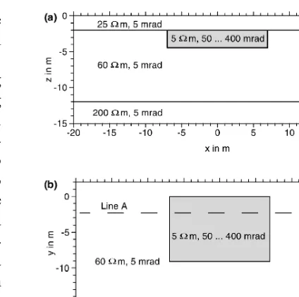
To investigate the ambiguity of the data, forward modelling was performed. The model shown in Fig. 8 consists of three layers: the top layer with a resistivity of 25 V m, a second layer with 60 V m and the underlying halfspace with 200 V m. The phase angles are chosen to be 5 mrad. The waste filled cell is designed as a
Ž .
Fig. 8. Three layer model with embedded waste body. a
Ž .
Vertical section at Line A. b Horizontal plane at a depth of 4 m.
rectangular body situated in the second layer with a resistivity of 5 V m and phase angles of 50, 130, 200, 300 and 400 mrad.
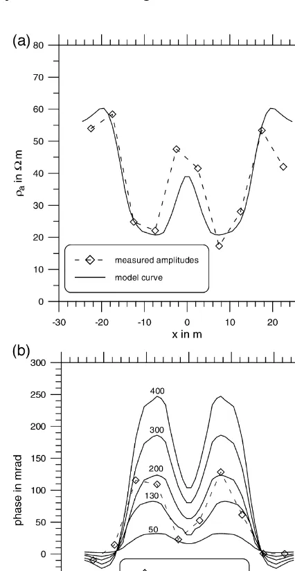
In the first step, 2-D models were run assum-ing an infinitely long trench. In Fig. 9a, the calculated and measured apparent resistivities are compared at the position of line A for a dipole separation of 20 m. The corresponding results for the different phase angles are shown in Fig. 9b. Both the measured and the calculated phase curves show two positive anomalies at the edges of the trench and a minimum in the centre of the structure. The best fit is achieved with an intrinsic phase angle of 200 mrad.
In the second step, 3-D models were run assuming a finite extent of the waste body in y-direction as indicated in Fig. 8b. Though the general shape of the resulting anomalies is com-parable to those from 2-D modelling, the central minimum becomes deeper reaching even nega-tive apparent phases, and the fit with the
mea-Ž .
resis-tivities of the layers have been chosen from the inversion result the measured resistivity ampli-tudes are also well fitted by the 2-D and 3-D
Ž .
models see Fig. 9a, Fig. 10a .
This modelling experiment has shown that the measured IP data can be confirmed if the waste body is located at the known depth, and if an extremely high intrinsic phase value is as-sumed. The inversion starting with a back pro-jection and searching for a smooth model yields
Fig. 9. Result of 2-D modelling and measured values for a
Ž .
dipole separation of 20 m. a Amplitude of apparent
Ž .
resistivity. b Phase lag.
Fig. 10. Result of 3-D modelling and measured values for
Ž .
a dipole separation of 20 m. a Amplitude of apparent
Ž .
resistivity. b Phase lag.
an equivalent model fitting the data, but the conductive, polarizable structure is located at a greater depth.
8. Comparison with other methods
sys-tems presently available, and to target areas of
Ž .
research Pellerin and Alumbaugh, 1997 . The comparison of the results of 11 different electromagnetic and electrical methods reveals
Ž .
that radiomagnetotellurics RMT , electrical re-sistivity and IP have presently the best potential to resolve buried waste material at CTP. Since an IP survey includes resistivity measurements the comparison is focused on RMT and IP. The radiomagnetotelluric survey covers nearly the same area as the IP survey. The results
pub-Ž .
lished by Tezkan and Dautel 1997 show a plan view of the resistivity at the LOP which was derived by a 2-D inversion of measurements at four frequencies at different lines. Regarding the location of anomalies and the determined values, the resulting resistivity images at a depth of 4 m from both IP and RMT are similar to a large extent. The phase image provided by the IP survey yields additional information to char-acterize the conductive zones. Large phase val-ues refer to the diffuse occurrence of metallic material in the waste.
The vertical sections at line A show for both methods the true horizontal extent. The cap thickness is well resolved by RMT and by the phase image of IP. Though overestimated, the vertical extent of the waste body can be better recognized in the images generated by 3-D in-version of IP data. The underlying Snake River basalt causes the high resistive region beneath the waste, which is missing in the RMT image because signals at sufficiently low frequencies were not available.
9. Discussion and conclusions
Anomalous responses of both resistivity and polarization are noted at the INEL CTP. Eleven parallel lines of dipole–dipole data have been acquired. Apparent resistivity is observed to decrease by a factor of 2 to 3 with respect to background, while apparent phase angle in-creases by a factor of 20 to 30. Furthermore, conductivity anomalies are present which are
unrelated to the presence of simulated waste. The polarization response is large, limited, and spatially correlated with the simulated waste.
An algorithm based on the SIRT and a finite difference forward modelling has proven to be a suitable tool for 3-D inversion of IP data. The algorithm, which works with complex conduc-tivities, uses the directly measured quantities of resistivity amplitude and phase shift as input data. The resulting 3-D model may be presented as horizontal or vertical resistivity and phase sections.
The contours and the top of the waste zone are well resolved. The bottom is detected, but the depth is overestimated by both resistivity and phase images. The inversion algorithm can not overcome the ambiguity of IP data.
The algorithm is easily implemented even for large data sets and grids. The SIRT has a slow convergence rate, but the application of a back projection yields a favourable starting model and ensures a reliable result after few iterations. Inversion of a data set of 640 configurations and a finite difference grid with more than 30,000 nodes requires about 6 h. The 3-D inversion procedure for large IP data sets should be accel-erated to enable field processing in a reasonable time. A comparison with alternative inversion procedures for complex electrical resistivity data
Že.g., Kemna and Binley, 1996 should be per-.
formed to show the advantages of each algo-rithm concerning speed, accuracy and power of resolution.
The presented modelling and inversion algo-rithms can be used for conventional resistivity measurements if the phase information is
ig-Ž .
nored Schulze et al., 1996 . The use of real instead of complex arithmetic considerably ac-celerates the processing.
points per day, including weather delays and logistical interruptions. The maximum produc-tion rate was 4 lines per day. A more rigorous
Žand less experimental implementation of these.
conventional means might achieve a sustainable data acquisition rate of 6–8 lines per day at a cost of roughly US$200–300 per line, or US$3.50 to US$5.50 per datum. The widespread use of this method requires development of a cost-effective, rapid IP data acquisition system using multielectrode and multichannel technol-ogy. We speculate that conventional galvanic IP data might be obtained in small-spacing surveys at a cost improvement of better than an order of magnitude compared to present methods.
Acknowledgements
We gratefully acknowledge field work assis-tance from Mr. Karl Merz of Cornell University and Ms. Suzan Frangos. The work was per-formed under the auspices of the Very Early
Ž .
Transient Electromagnetics project VETEM . A.W. was financially supported by the Deutsche Forschungsgemeinschaft through a Werner– Heisenberg–Stipendium.
References
Angoran, Y., Fitterman, D.V., Marshall, D.J., 1974. In-duced polarization: a geophysical method for locating
Ž .
cultural metallic refuse. Science 184 4143 , 1287– 1288.
Bleil, D.F., 1953. Induced polarization: a method of geo-physical prospecting. Geophysics 18, 636–661. Borner, F., Jung, F., Schon, J., 1991. Complex electrical¨ ¨
conductivity of KTB samples in the frequency range between 10y3 and 104 Hz—first results. Scientific
Drilling 2, 101–104.
Collett, L.S., 1990. History of the induced-polarization
Ž .
method. In: Fink et al. Eds. , Induced Polarization: Applications and Case Histories. Investigations in Geo-physics, No. 4, SEG, Tulsa, pp. 5–21.
Dey, A., Morrison, H.F., 1979. Resistivity modeling for arbitrarily shaped three-dimensional structures. Geo-physics 36, 753–780.
Dines, K.A., Lytle, R.J., 1979. Computerized geophysical tomography. Proceedings IEEE 67, 1065–1073. Frangos, W., 1990. Stable-oscillator phase IP systems. In:
Ž .
Fink et al. Eds. , Induced Polarization: Applications and Case Histories. Investigations in Geophysics, No. 4, SEG, Tulsa, pp. 79–90.
Frangos, W., 1997. IP and resistivity survey at the INEL Cold Test Pit. Expanded Abstr., 10th SAGEEP meet-ing, Reno, NV, pp. 817–824.
Frangos, W., Andrezal, T., 1994. IP measurements at contaminant and toxic waste sites in Slovakia. Ex-panded Abstr., Summer IP Workshop, Tucson. Grow, L.M., 1982. Induced polarization for geophysical
Ž .
exploration. The Leading Edge, 1 6 , 55–56 and 69–70. Kemna, A., Binley, A., 1996. Complex electrical resistiv-ity tomography for contaminant plume delineation. Pro-ceedings of the 2nd Meeting of the Environmental and Engineering Geophysical Society, Nantes, pp. 196–199. Olayinka, A.I., Weller, A., 1997. The inversion of geoelec-trical data for hydogeological applications in crystalline basement areas of Nigeria. J. Appl. Geophys. 37, 103– 115.
Oldenburg, D.W., Li, Y., 1994. Inversion of induced polar-ization data. Geophysics 59, 1327–1341.
Pellerin, L., Alumbaugh, D.L., 1997. Tools for electro-magnetic investigations of the shallow subsurface. The Leading Edge 16, 1631–1638.
Pelton, W.H., Ward, S.H., Hallof, P.G., Sill, W.R., Nel-son, P.H., 1978. Mineral discrimination and removal of inductive coupling with multifrequency IP. Geophysics 43, 588–609.
Seigel, H.O., 1959. Mathematical formulation and type curves for induced polarization. Geophysics 24, 547– 565.
Schlumberger, C., 1920. Etude sur la prospection elec-trique du sous-sol. Gauthier-Villars et Cie., Paris. Schulze, K., Seichter, M., Seuffert, M., Kumpel, H.-J.,¨
1996. High resolution electrical measurements at a test site near Julich, Germany. Expanded Abstract, 58th¨
EAGE Conference, Amsterdam.
Sumner, J.S., 1976. Principles of Induced Polarization for Geophysical Exploration. Elsevier, Amsterdam.
¨
Tezkan, B., Dautel, S., 1997. Uber RMT-Messungen auf einer kunstlichen Altlast in IdahorUSA. DFG-Sonder-¨
band II, 4. DGG-Seminar Umweltgeophysik, pp. 131– 142.
van der Sluis, A., van der Vorst, H.A., 1987. Numerical solution of large, sparse linear algebraic systems arising
Ž .
from tomographic problems. In: Nolet, G., Ed. , Seis-mic Tomography. Reidel, Dordrecht, pp. 49–83. Vanhala, H., Soininen, H., Kukkonen, I., 1992. Detecting
van Voorhis, G.D., Nelsen, P.H., Drake, T.L., 1973. Com-plex resistivity spectra of porphyry copper mineraliza-tion. Geophysics 38, 49–60.
VETEM, 1996. The VETEM web site at http:rr vetem.lbl.gov presents data from the EMID project and descriptions of the surveys performed.
Weller, A., 1986. Berechnung geoelektrischer Poten-tialfelder mit dem Differenzenverfahren. Freiberg. Forschungsh. C 405, 68–122.
Weller, A., Borner, F.D., 1996. Measurements of spectral¨
induced polarization for environmental purposes. Envi-ronmental Geology 27, 329–334.
Weller, A., Seichter, M., Kampke, A., 1996a. Induced-polarization modelling using complex electrical con-ductivities. Geophys. J. Int. 127, 387–398.
Weller, A., Gruhne, M., Seichter, M., Borner, F.D., 1996b.¨