Measuring the influence of Canadian
carbon stabilization programs on natural
gas exports to the United States via a
‘bottom-up’ intertemporal spatial price
equilibrium model
qSteven A. Gabriel
a,b,U, Shree Vikas
b, David M. Ribar
ca
Department of Engineering Management and Systems Engineering, The George Washington Uni¨ersity, Washington, DC 20052, USA
b
ICF Consulting, 9300 Lee Highway, Fairfax, VA 22031-1207, USA
c
Amtrak, 10 G Street, NE, Washington, DC 20002, USA
Abstract
In this paper, we present the results of a study of the impact of Canadian carbon stabilization programs on exports of natural gas to the United States. This work was based on a study conducted for the US Environmental Protection Agency. The Gas Systems
Ž .
Analysis model GSAM , developed by ICF Consulting for the US Department of Energy, was used to gauge the overall impact of the stabilization programs on the North American
Ž .
natural gas market. GSAM is an intertemporal, spatial price equilibrium SPE type model of the North American natural gas system. Salient features of this model include characteri-zation of over 17 000 gas production reservoirs with explicit reservoir-level geologic and economic information used to build up the supply side of the market. On the demand side, four sectors } residential, commercial, industrial and electric power generation } are characterized in the model. Lastly, both above and below ground storage facilities as well as a comprehensive pipeline network are used with the supply and demand side
characteriza-q
Ž .
Note that an earlier, reduced form of this paper appeared in Gabriel et al. 1998a .
U
Corresponding author. ICF Consulting, 9300 Lee Highway, Fairfax Virginia 22031]1207, USA
Ž .
E-mail address:[email protected] S.A. Gabriel .
0140-9883r00r$ - see front matterQ2000 Elsevier Science B.V. All rights reserved.
Ž .
signed the Framework Convention on Climate Change. According to the agree-ment, countries promised to increase public awareness about the hazards of climate change and agreed to collaborate to alleviate the problem.
In the spirit of the contract, Canada, along with other nations, established a goal to stabilize greenhouse gas emissions by the year 2000 to the level emitted in 1990. This objective was to be governed in Canada by the National Action Program on
Ž .
Climate Change NAPCC . NAPCC was formed from federal, provincial and territorial governments to develop strategies to reduce carbon emissions and to monitor progress. Canada’s Climate Change Voluntary Challenge and Registry,
Ž .
Inc. VCR, Inc. , a key component of NAPCC, was created in February 1995 and was designed to record the efforts of private and public sector organizations in reducing greenhouse gas emissions.
The purpose of the study presented in this paper was to analyze the effects of the carbon stabilization efforts of the VCR, Inc. on Canadian exports of gas to the United States. Recently, there have been a good number of studies geared at North
Ž
American CO policy modeling. Examples of these works include Kanudia and2
.
Loulou, 1998a,b,c,d; Loulou et al., 1996; Loulou and Kanudia, 1997, 1998 , as well
Ž .
as Chung et al., 1997 . This paper distinguishes itself from these works in the level of detail on the upstream and downstream sides of the market for the model used,
Ž .
that is, the Gas Systems Analysis Model GSAM .
GSAM characterizes the supply side of the North American natural gas market by over 17 000 individual gas reservoirs each with explicit geologic and economic variables. This level of detail allows for reasonable simulation of the economic behavior of individual reservoir operators. This approach, while numerically chal-lenging allows for a more realistic modeling of the supply side than the traditional regional level approach. The result is that supply curves for the 24 supply regions are more responsive to market conditions and technologies than would otherwise be the case.
On the downstream side of the market, GSAM consists of 16 North American demand regions with 79 transportation links connecting supply and demand re-gions. The demand is then brought together with supply in an integrating linear
Ž . Ž .
of gas as well as the demand for gas at the node. For demand regions, inflows of gas to meet demand in all four sectors can arrive by pipeline from other regions,
Ž
from underground gas storage reservoirs, or from peaking supply propanerair,
. Ž
LNG . The LP considers both the operational as well as investment capacity
.
expansion decisions related to the natural gas system as a whole and is based on the concept of maximizing total surplus.
Canada’s role in the North American market has become increasingly substan-tial in recent years. Since 1990, 43% of US growth in gas consumption has been supplied by imports from Canada. During this period, Canadian exports to the US
Ž .
have doubled Energy Information Administration, 1991, 1997 . The Canadian natural gas market has grown significantly in the 1990s. Canadian marketed gas
Ž .
production in 1996 was 5.7 Tcf trillion cubic feet according to the Canadian
Ž .
Association of Petroleum Producers CAPP , a 56% increase from 1990. A share of this growth is due to Canada’s growing exports to the US market. In addition, increased demand in Canada is also a factor. The Canadian domestic demand has
Ž
increased 19% since 1990 to a level of 2.6 Tcf in 1996 Oil & Gas Journal Energy
.
Database, 1997 .
The long-term future of Canada’s natural gas industry appears prosperous as well. Canada’s growing role as an exporter coupled with its internal growth has caused many to forecast an optimistic future for Canadian gas. Natural Resources Canada, in their 1997 outlook, projects an average annual growth rate of 0.8% for
Ž .
natural gas demand over the next 25 years NRCAN, 1997 . Canada currently contributes 13% to US gas demand through exports, and this share is expected to
Ž .
increase Energy Information Administration, 1997 . Some analysts are concerned that at some point, the increased demand for gas in Canada to assist in the carbon emission stabilization effort could decrease Canadian natural gas exports to the US and increase gas prices in key US markets.
2. Stabilizing carbon emissions
Carbon dioxide, methane and nitrous oxide play a critical role in regulating the temperature on the earth’s surface. These ‘greenhouse gases’ absorb infrared light and trap heat that would otherwise escape through the atmosphere and dissipate into space. This process is natural and necessary to our habitat. Scientists have hypothesized for many years that increasing levels of these gases in the atmosphere will ultimately lead to a warmer global climate. In addition, it has been shown that these gases can take thousands of years to cycle out of the atmosphere. Each year, human activities are releasing more and more greenhouse gases into the atmo-sphere. Consequently, many experts believe that even at current levels anthropo-morphic greenhouse gas emissions could cause a dramatic shift in the earth’s
Ž .
climate. Carbon-based gases CO and methane , constitute by far the largest2
percentage of man-made greenhouse gases in the atmosphere.
3. Role of the VCR program
The goal of the VCR program is to reduce the projected carbon emissions in the year 2000 to the level emitted in 1990. The program, which was only 2 years old at the time of this writing is a good first step, but it has two noticeable weaknesses.
Ž
First, while the VCR, Inc. includes many members over 70% of Canada’s
green-.
house gas emissions are represented , it is still voluntary and does not impact all Canadian organizations. Second, the VCR, Inc. has no official regulations or policies. Each member devises their own plan to control carbon emissions, and is responsible for achieving their goals. As member activities are voluntary, some members may be less aggressive with their actions than others. Fig. 1 shows recent forecasts of carbon emissions from NRCAN.
Although it does not appear that stabilization will be met with the VCR, Inc. program alone, progress is being made. As the chart depicts, the projected carbon emissions for 2000 have decreased over 6% from the 1994 to 1997 NRCAN forecasts. Therefore, the organizations that are being established appear to have made an impact, at least in the forecasters’ minds. The focus of this study, however,
is not on whether stabilization will be achieved, but what effects the Canadian measures will have on the overall North American natural gas market. Controlling carbon emissions in Canada will obviously have an effect on the Canadian market, but it could also alter the US gas and electricity markets.
There are five strategies frequently employed by the VCR, Inc. to reduce carbon emissions. These include: energy efficiency projects, demand side management, fuel substitution, process redesign and implementation of offset initiatives. The most common strategy for reducing carbon emissions is the use of energy efficiency projects. Examples of these projects include equipment upgrades, fleet downsizing and cogeneration; but they can include any method that implements a better, more efficient, usage of energy. The second strategy, demand side management, comes from a joint effort between the electric utilities and their stakeholders to better manage carbon emissions. The third strategy, fuel substitution, involves replacing cheaper fossil fuels with cleaner, although more expensive, burning fuels, such as renewables or natural gas. The process redesign strategy involves organizations developing methods to reduce carbon emissions during manufacturing. The final strategy is the implementation of offset initiatives, particularly in the forestry, pulp and paper sectors.
This study addresses only the third strategy of reducing carbon emissions based on replacing fossil fuels used in electrical power generation with cleaner alterna-tives. The fossil fuels that we have considered are coal, natural gas, residual fuel oil and distillate, and we have considered stabilization for the year 2010. Also, it should be noted that consistent with the EPA study performed by ICF Consulting
ŽICF Kaiser, 1997 , only stabilization efforts in Canada were considered. The.
analysis of how stabilization efforts in the US as well might affect the natural gas industry is potentially the subject of future work.
4. The Gas Systems Analysis Model
GSAM is a modular, reservoir-based model of the North American natural gas system, developed by ICF Consulting under the sponsorship of the US Department
Ž .
of Energy DOE . GSAM represents a flexible, sophisticated approach for model-ing supply, demand and transportation issues in the North American natural gas market. It has undergone a comprehensive, in-depth review by industry, govern-ment and academic peers. It is reliable and efficient in analyzing the broad range of issues being addressed in this study and has been successfully used to evaluate various upstream and downstream issues in natural gas, including consideration of alternative technology scenarios, market conditions and public policy initiatives on
Ž
US gas supplies and the strategic decisions made by oil and gas companies see for example Becker et al., 1995; Gabriel et al., 1996, 1997, 1998a; Vikas et al., 1996,
.
1998 .
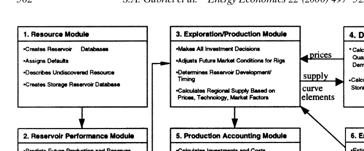
Fig. 2. Major components of the Gas Systems Analysis Model.
of potential North American gas supplies are specified at this level of disaggrega-tion, GSAM is free from restrictive assumptions such as regional average supply curves normally imposed by traditional gas market models.
On the downstream side of the market, GSAM consists of 16 North American demand regions with 79 transportation links connecting supply and demand
re-Ž
gions. These links represent collections of pipelines serving the regions or
inter-.
mediate points in question. The demand for natural gas is characterized by four sectors: residential, commercial, industrial and electric power generation. Com-bined with multiple seasons and years, the result is a model fairly rich in detail. The upstream and downstream sides of the market are brought into balance by an integrating LP which seeks to maximize the sum of producer plus consumer surplus less transportation costs, resulting in equilibrium prices, quantities, and flows. Various GSAM sub-modules interact with each other in a manner illustrated in Fig. 2 to perform the aforementioned activities.
4.1. The modeling of the supply side of the natural gas market
The modeling of the supply side of the natural gas market in GSAM is based on simulating exploration and production activities of typical production reservoir operators. The economic behavior of these reservoir operators is modeled in the context of given prevailing market conditions and technologies. The regional
Žaggregate supply curves are then created by summing up the production respon-.
ses from each of the reservoirs analyzed. In this way, GSAM builds regional supply curves from the ‘bottom-up’.
The exploration and production algorithm used in GSAM is a play1 level
Ž .
approach based on the work of L.P. White White, 1981 . In this methodology,
1
exploration activities are simulated using both geologic and economic data pertain-ing to the play. There are four main steps in simulatpertain-ing the exploration process over time for each play:
Step 1: Determine the number of undiscovered accumulations2 based on US
Ž .
Geological Survey USGS estimates,
Step 2: Rank all the undiscovered drilling accumulations based on an expected profitability index taking into account the probability of drilling dry holes,
Step 3: Perform exploratory drilling until either a rig utilization constraint is encountered or until the complete USGS-estimated economic resource for the accumulation has been found,
Step 4: Update in a Bayesian manner, the probability of finding accumulations in a play based on the already discovered resource.
For exploration to be conducted, the expected value of the next discovery must
Ž .
exceed the full cost of finding natural gas including dry holes , and ultimately
Ž .
developing and producing the potential discovered reservoir s . Once a reservoir has been discovered, development and production from that reservoir must gener-ate expected revenues to cover the investments, operating costs and risks of development. Each investment decision is approached from the point of view of an operator determining if the investment is warranted. These evaluations integrate detailed information on reservoir geology, technology, productivity, costs and market prices consistent with operator decision-making. Once the exploration decisions are made, development economics are conducted on a sunk-cost basis to account for investments already made.
Ž .
Compared with the approach in White, 1981 , our approach ranks the undiscov-ered accumulations based on expected profitability as opposed to expected volume. Our approach is appropriate if one is modeling reservoir operators behaving in a rational economic manner whose activities are profit-motivated. In addition, our
Ž
method uses rig constraints as opposed to budget constraints as used in White,
.
1981 . We believe that our approach is more realistic since an attractive drilling prospect could generate sufficient funding and thereby avoid the need for a budget limit but would not be able to bypass the physical constraint on the actual number of existing plus potential available drilling rigs.
4.1.1. Modeling the effect of technology on exploration and de¨elopment decisions
To model the economic behavior of the typical reservoir operator, GSAM considers both the discovered as well as the proven yet undiscovered resource at the operator’s disposal. Based on an expected net present value analysis3, the operator may decide not to proceed with exploration due to unfavorable economics. However, if the decision to explore makes economic sense, for proven
undiscov-2
An accumulation is defined as either a single reservoir or an aggregation of reservoirs.
3
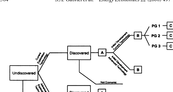
Fig. 3. GSAM decision tree for exploration and production activities.
ered hydrocarbons, the operator can use either current or advanced technology.
Ž .
Once the resource is discovered either by current or advanced methods , a second series of profitability calculations are performed to determine if development of the resource should proceed. If the decision to develop is economically viable, again the operator can use current or advanced methods based on their relative costs. The development decision is made for each individual reservoir at the
Ž
paygrade level GSAM uses three paygrades per reservoir to account for the
.
heterogeneity of the resource . This decision process is depicted in Fig. 3.
4.1.2. Modeling full-cycle costs for E & P operators
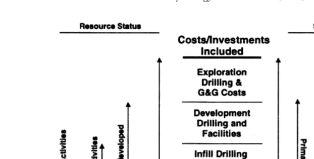
As shown in Fig. 4, GSAM models the resource and associated costs at every stage of reservoir exploration andror development. On the left-hand side of this figure, we show resource status and on the right we indicate the stage of reservoir
Ž .
development. The height of the arrows on either side coincide with the height of the costs column to indicate which costs are applicable for each category con-sidered. For example, proven undiscovered resource undergoes all stages of devel-opment that is: exploration, primary and secondary develdevel-opment, recompletion,
Ž .
and shut-in. However, producing reservoirs the left-most resource status only incurs operating costs and taxes to determine if continued production or shut-in is appropriate.
4.1.3. The MASP concept in GSAM’s E & P module
In determining if a particular exploration or development project is economically
Ž .
Fig. 4. GSAM exploration and production costing approach.
price at which exploration andror development of a reservoir would be undertaken
Ži.e. gas price at which hurdle rate is met . It is important to note that the MASP is.
a function of the market gas price, which in turn is dependent on the supply side of the market of which the MASP has a significant effect. To account for this interdependence, the MASP is interpolated or extrapolated at various market gas prices and market conditions. As shown in Fig. 5, the MASP is also discounted over time.
In GSAM, the MASP is compared with the market equilibrium price and when the MASP is less than or equal to the price, the operator selects appropriate explorationrdevelopment options, otherwise, no activity results. Estimates of mar-ket equilibrium prices are determined via the integrating model of GSAM as described in the next section. This is the main connection between the supply and demand side models of the market in GSAM.
Fig. 5. Minimum acceptable supply price.
4.2. The modeling of the demand and transportation sides of the natural gas market
Fig. 6. A typical curve discretization.
including both firm and interruptible demand in the relevant sectors. To capture the effects of seasonality, seasonal load factors are employed. These factors, which vary by region, indicate the ratio of gas demand per day in a particular season relative to an average day in the year.
The demand is then brought together with supply in an integrating LP. This LP
Ž .
balances for each node region , season, and year, the supply of gas as well as the demand for gas at the node. For demand regions, inflows of gas to meet demand in all four sectors can arrive by pipeline from other regions, from underground gas
Ž 4.
storage reservoirs, or from peaking supply propanerair, LNG . The LP considers
Ž .
both the operational as well as investment capacity expansion decisions related to the natural gas system as a whole. To incorporate both the supply and demand sides in a linear programming format, the relevant demand and supply functions
Ž .
are discretized and approximated usually in a step-function manner .
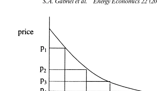
For the residential and commercial sectors, demand at a particular node and
Ž .
time period is modeled as a log-linear i.e. constant elasticity function of popula-tion, GNP and gas price. This log-linear curve is then approximated by a step
Ž .
function formulation based on small under $0.10 price increments. A sample approximation to the area under a demand curve is with five price-quantity increments shown in Fig. 6.
Thus, the total demand for a region and time period is given by
TDs
Ý
qii
and
q
Ž .
D z dz(
Ý
q pH
i i0 i
4
With a fine enough discretization, this scheme can provide a useful approximation to a demand curve and is easy to incorporate in a linear programming format. While population and GNP are part of the demand equations for gas, they enter only as exogenous factors and it is the price of gas that is calculated endogenously in GSAM.
The demand for natural gas in the industrial sector is modeled in a similar step-function manner except that the breakpoints refer to the prices of the alternate fuels used in this sector. Besides natural gas, the demand model takes into account, low sulfur residual oil, high sulfur residual oil and distillate fuel. In this way, the model simulates the competition between gas and alternative petroleum products to satisfy industrial needs.
In the electrical power sector, demand is broken down into power plants by fuel type and seasonal pattern of natural gas usage. There are separate demand variables for nuclear, coal, hydrorother, combined cycle, low sulfur residualrgas, high sulfur residualrgas and distillatergas plants.
To transport the gas, a network system is modeled wherein the links represents aggregates of actual pipelines and the nodes refer to supply, demand, or
intermedi-Ž .
ate regions. Typical information on each pipeline link either existing or potential
Ž .
includes the following MCFs1000 cubic feet, MMCFs1 000 000 cubic feet :
v the start and end node for the link;
v the link capacity in MMCFrday;
v the levelized investment costs5 in $rMCF;
v the fixed operations and maintenance costs in $rMCF;
v the variable operations and maintenance costs in $rMCF;
v the first year that the link is available; and
v the fuel loss along the link in %.
The main set of constraints for this LP are material balance at each node, time and season, that is, what comes into a node must equal what goes out. The inflow
Ž
to a node is the sum of flows from other nodes less the fuel needed to run
.
compressors and gas that may be lost due to leaks , gas extracted from available storage reservoirs and the supply of gas available at the node from production reservoirs as well as propane, LNG sites or extra supply projects. In terms of what can leave a node, the model considers the flow of gas to other nodes, gas that is injected into storage sites, as well as customer demand for that node. This demand includes the residential, commercial, industrial and electric power generation sectors. The LP considers the economics of adding andror using pipeline, storage or other capacity to balance supply and demand. In addition to the material balance constraints, there are also additional realistic constraints that govern how much gas can move along the network; examples of these constraints include:
5
v the fuel usage in %; and
v the expected number of years in the life of the storage reservoir.
It is important to note that these values are not fixed a priori but are generated
Ž .
within GSAM’s Storage Reservoir Performance Module Vikas et al., 1996 which takes into account various geological, technological and economic conditions for each storage reservoir. As a result of this rich detail on storage reservoirs, the integrating LP is quite useful for gauging the importance of alternative storage technologies and policies. In addition, the integrating LP can measure the relative importance between using storage reservoirs or building additional pipeline to satisfy the larger daily gas requirements of the winter season.
4.3. The integration of upstream and downstream acti¨ities
The integrating module of GSAM is based on the well-known spatial price
Ž . Ž .
equilibrium SPE model as described in Takayama and Judge, 1971 . It differs from the traditional model in several important ways which we describe below in addition to briefly reviewing SPE.
The SPE problem is to find equilibrium prices and quantities in a set of geographically disperse regions as well as equilibrium flows between these regions. SPE is based on maximizing the total welfare given as
Ž .
Ws
Ý
W yi i,xii
Ž .
whereW yi i,xi, yi, xiare, respectively, the welfare, the demand and the supply for
Ž . Ž .
region i. If the inverse demand and inverse supply functions are given,
respec-Ž . i Ž .
tively, as pisD yi i,p sS xi i, then we define the quasi-welfare function as
yi xi i
Ž .
W yi i,xi s
H
p di hiyH
p djiUnder an assumption that the total welfare is the sum of the regional welfares6, we have the total welfareW given as
Ž .
Ws
Ý
W yi i,xii
Additionally, if xi j, ti j measure, respectively, the flow of gas from region i to region j and the associated transportation costs between these markets, then we
Ž .
can define the net quasi-welfare function Takayama and Judge, 1971 as
yi xi i
this form is also known as the net social payoff NSP which maximizes the sum of producers’ and consumers’ surplus after deducting for transportation costs
ŽSamuelson, 1952; Labys and Pollak, 1984 ..
A common approach is to maximize this net quasi-welfare function subject to constraints forcing no excess demand, allowing for excess supply possibility, regio-nal consumer and production equilibria conditions as well as locatioregio-nal price equilibrium conditions. For some recent examples of variations of this approach in
Ž
the energy industry as well as summaries, see Greenberg and Murphy, 1985; Weyant, 1985; Yang and Labys, 1985; Takayama and Labys, 1986; Murphy, 1987;
.
Labys and Yang, 1991 .
Ž .
This formulation is based on the assumption that the inverse supply and demand functions are integrable. On the gas supply side of the market, this assumption may be violated for at least two reasons. First, the production levels are affected by the amount of available drilling rig capacity in a region. When prices differ between supply regions, there is an economic incentive to move drilling rigs, thus changing the effective regional rig capacity and ultimately drilling and produc-tion levels in the region. In this way, on the supply side of the market, we see that there is dependence between regions not necessarily in a symmetric way. Thus, by
Ž .
the symmetry principle Ortega and Rheinboldt, 1970 , the supply functions may not be integrable.
Second, cross-regional influence can also be important in the presence of environmental constraints imposed on the producers of gas. The effect of
environ-Ž .
mental regulations proposed or actual has different levels of influence on different regions. More stringent regulations have the effect of raising the environ-mental cost of compliance and thus the break-even price for reservoir operators. Consequently, regions with relatively less restriction could appear more attractive for the operators thereby affecting the production levels of a region.
On the demand side, the demand for gas is affected not only by the own regional prices but also by the prices in regions that are connected via the pipeline system.
6
Besides the interregional dependence for supply and demand curves, there is also intertemporal dependence in the natural gas market. In particular, if we ignore the interregional dependence and denote the price in supply region i at
t t t tŽ 1 2 t.
time t as pi with associated supply as Si then we see that SisS pi i,pi, . . . ,pi . It is necessary to know what the prices are from the current as well as all previous time periods in evaluating the current regional supply. This dependence is due to the fact that the price in earlier time periods affect the amount of gas that is produced out from the reservoirs in later periods. This in turn affects how much pressure and resource is left in the reservoir for the second time period. Thus, one
Ž
needs to know the complete history of what was produced as well as any new
.
drilling activity in evaluating the supply for the current time period.
4.4. Mathematical form for GSAM’s equilibrium problem
A version of the standard total surplus maximization problem but with operatio-nal and investment constraints as well as discounting over time is used to generate equilibrium prices and quantities in GSAM. A somewhat stylized form of the associated optimization problem is given below.
qnt s
Ž . Ž .
max
Ý Ý Ý
dt sž
H
TDn t s z dz/
y½
Ý Ý
OC dt s t sqÝ
IC dt t5
2o
s n s
t t t
subject to operational and in¨estment constraints
where
OCt s is the system operating costs in time t, season s, ICt is the investment costs in time t,
Ž . Ž
TDn t s . is the total demand curve for gas in node n, time t, season s summed
.
across sectors ,
dt s, dt are appropriate discounting factors.
Table 1
Carbon emission factors in the electric utility sector
Fuel type Millions of tons of CO2rTeraWatthour
Coal 1.20
Oil 0.83
Gas 0.40
for example, the total demand is given as follows:
qnt s season s, in increment i, and the associated price for this increment; see Appendix
Ž .
A for further details. The objection function in Eq. 2 is related to the objective
Ž .
function for the standard total surplus maximization problem Eq. 1 by noting that
Ž
the operating costs term OCt s includes the cost of supply production,
peak-shav-.
ing, and extra projects , approximating the producer surplus. In addition, the operating costs term includes pipeline transportation costs, and storage operations costs. The investment costs term, ICt, considers capacity expansion for pipelines, electrical power plants, as well as storage reservoirs.
5. The carbon stabilization study results
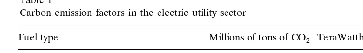
Before modeling a case corresponding to carbon stabilization, it was first necessary to decide upon a method for estimating carbon emission levels. Given that carbon emissions are directly proportional to fuel consumption, a carbon
Ž . Ž
emission factor Table 1 was determined for each fuel type with input from
.
Natural Resources Canada .
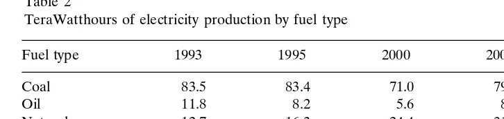
To evaluate the effect of Canadian carbon stabilization programs on gas exports to the United States, we compared the outputs from GSAM using a base case and three carbon stabililization cases. In all cases, we made use of electricity produc-tion figures supplied by NRCAN by various fuel types. These figures are shown in Table 2 below7,8,9.
7
NRCAN’s data were interpolated for 1993, but actual figures were made use of for the remaining years. For hydrorother power in 1993 and nuclear power for 1995, the model was allowed to deviate somewhat from the NRCAN values due to avoid internal infeasibilities that were encountered.
8
GSAM’s downstream model used the following years in its integrating linear program: 1993, 1995, 2000, 2005, 2010
9
Since the only differences between the base case and these stabilization cases were the stabilization activities, we can attribute the change in the solution to the stabilization effects10. This difference is thus an estimate of the influence of these measures in Canada on the North American natural gas market. The various levels of the CO emissions constraint, applied to the year 2010 for the Canadian2
Electrical Power Generation Sector, are shown in Table 3. The nominal target
Ž115.12 short tons was based on the 1990 baseline figures from the Canadian.
Ž .
Electricity Association CEA with 10 participating utilities. CEA represents 11 major utilities involved in the VCR program which constitutes over 95% of the
Ž
total carbon emissions from fossil fuel fired generation in Canada Canadian
.
Electricity Association, 1996 and hence their forecast can be considered appropri-ate.
Based on discussions with energy professionals at NRCAN and elsewhere in Canada, the base case assumptions included:
v Using coal electricity production values from Table 2 for 1993]2010.
v Using nuclear, hydrorother, gas, and oil electricity production values from
Table 2 for 1993 and 1995 only7, but allowing the model to select appropriate
Table 3 CO limits2
CO limit2 Description
104.44 short tons Most restrictive stabilization case
115.12 short tons Nominal target stabilization case
126.90 short tons Least restrictive stabilization case
Ž .
99999.0 short tons No stabilization case base case
10
Fig. 7. Electric generation sector in Canada}base case.
values for nuclear, hydrorother, gas, and oil to match total electricity production in the years 2000, 2005 and 2010.
Forcing the model to prohibit additional nuclear or hydrorother capacity from 1995 or later.
Not imposing a CO emissions constraint on Canada.2
The carbon stabilization cases’ assumptions included:
Using coal electricity production values from Table 2 for 1993]1995, but al-lowing the model to select appropriate values for the years 2000, 2005 and 2010,
Using nuclear, hydrorother, gas and oil electricity production values from Table 2 for 1993 and 1995 only7, but allowing the model to select appropriate values for nuclear, hydrorother, gas and oil to match total electricity production in the years 2000, 2005 and 2010,
Forcing the model to prohibit additional nuclear or hydrorother capacity from 1995 or later,
Ž
Imposing a CO emissions constraint on Canada in the year 2010 which varied2
.
by stabilization case .
5.2. Summary of results
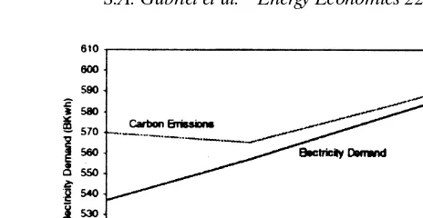
The carbon emissions and electrical demand levels for the Canadian electrical power sector under the most restrictive stabilization cases as well as the base case are shown in Figs. 7 and 8. While the base case shows an increase in both electricity demand as well as carbon emissions, the most restrictive stabilization case shows for the same electricity demand levels, an abrupt decline in carbon emission in 2010.11
11
One particularly interesting result from this study was that the CO2 limits imposed can have a significant impact on the regional results. In particular, eastern Canada, where there was a dramatic increase in demand for gas, was the most
Ž .
sensitive to the three stabilization limits imposed as compared with the base case . Other regions showed less variation in the results as a function of different CO2 caps. This points to the need to carefully estimate the stabilization limits due to their strong but regionally disparate influence.
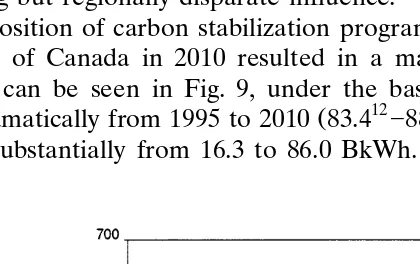
The imposition of carbon stabilization programs in the electrical power genera-tion sector of Canada in 2010 resulted in a major shifting of fuels used in this sector. As can be seen in Fig. 9, under the base case, the use of coal does not
Ž 12 .
change dramatically from 1995 to 2010 83.4 ]88.4 BkWh whereas the use of gas increases substantially from 16.3 to 86.0 BkWh. The most restrictive stabilization
Fig. 9. Electricity demand in Canada by fuel type}base case.
12
Fig. 10. Electricity demand in Canada by fuel type}most restrictive case.
case showed much more dramatic results, namely coal use dropped from 83.4]40.5 BkWh whereas gas increased significantly from 16.3 to 135.5 BkWh as shown in Fig. 10.
In terms of carbon emissions produced in the Canadian electrical power sector, as shown in Figs. 11]13, the contribution of coal diminishes somewhat between
Ž .
1995 and 2010 88]74% even under the base case. However, this decline is greatly accelerated under the most restrictive case showing a dramatic shifting towards gas and away from coal due to the lower emissions factor for gas. Note that oil does not play a significant role in this analysis. Fig. 11 shows the share of carbon emissions in 1995 for the fossil fuels considered. These shares are the same for
Fig. 12. Source of carbon emissions in the electric generation sector in Canada base case, 2010.
both the base and the most restrictive carbon stabilization case.
In contrast, in the year 2010, the share for coal drops significantly and the share for gas rises significantly due to carbon stabilization efforts that induce fuel switching as shown in Figs. 12 and 13.
The imposition of the CO emissions constraint in 2010 for the Canadian regions2 in GSAM resulted in a major shifting of the fuels in Canada used to produce electricity. These adjustments led to dramatic changes in imports and exports of gas between Canada and the United States and resulted, in some cases, in significantly elevated prices of natural gas in demand markets. As shown in Fig. 14, we see that in 2010, under the most restrictive stabilization case, Canada on the whole dramatically increased its imports from and cut back its exports to the US. In comparing the most restrictive stabilization case vs. the base case, we see that
Fig. 14. Net effects of carbon stabilization programs in Canada on national flows in 2010: most restrictive stabilization case}base case.
43213 Billion Cubic Feet more gas is in Canada. For the nominal and least restrictive cases, the net imports of gas from the US compared with the base case were, respectively, 334 and 211 BCF. It is interesting to note that while the CO2
Ž .
limit increased by only approximately 22% 126.90 short tonsr104.44 short tons , a
Ž
significantly greater need for gas in Canada resulted, namely, a 105% jump 432
.
BCFr211 BCF in net imports from the US.
The shifting CO limits caused some dramatic changes in the pipeline flows as2
might be expected. In particular, as shown in Fig. 15, as this limit became tighter
Žlower , more of the flow between the aggregated regions was directed towards.
eastern Canada, the major demand market for increased levels of gas in order to comply with stabilization.
Ž .
The increased demand for gas in eastern Canada and neighboring US regions resulted, under the most extreme stabilization, in some sizeable gas price increases in the US electric power sector. In particular, the largest increases in the US regional gas prices for 2010 were registered by the South Atlantic, New England and Middle Atlantic regions with increases of $0.20, $0.16 and $0.15, respectively. These price increases were matched by decreases in quantities demanded in these regions by 0.0, 6.5 and 28.4 BCF, respectively. The increased demand for gas in Canada also produced higher electric power sector prices for gas in Eastern Canada of about $0.62rMCF. The increased prices for combined GSAM demand regions are shown in Table 4 under the three stabilization cases. In addition, the increase in prices in the aggregated regions shown above were coupled with changes in demand quantities are also shown in Table 4. Again, it is eastern Canada that is most sensitive to the stabilization limit.
13
This figure of 432 is the increased levels of exports from the US to Canada less the decrease
Ž .
Fig. 15. Net effects of carbon stabilization programs in Canada on pipeline flows, 2010 } most restrictive case.
6. Conclusions
In this study we have shown how Canadian carbon stabilization programs can effect the entire North American natural gas system. We have made use of an intertemporal SPE model with production reservoir level detail on the supply side and seasonal, yearly, sectoral detail on the demand side. In addition, the demand side included storage reservoir and pipeline level inputs. The results indicate that stabilization programs can affect regions differently depending on the need for gas. Indeed, the regional prices and quantities as well as inter-regional flows can shift dramatically. We have seen that Eastern Canada had the most significant changes with several nearby US regions also being affected substantially. Lastly, we also observed that the value of the CO level imposed has influential effects on the2 results.
Acknowledgements
We would like to thank the following people: Benjamin Hobbs of The Johns Hopkins University for his comments regarding this paper, Anthony Zammarelli at the National Energy Technology Laboratory, US Department of Energy, for supporting GSAM, James Turnure at the US Environmental Protection Agency for funding work that formed the basis for this paper, Ashley Godell and Gary Guzman of ICF Consulting for their computational assistance and Neil McIlveen
´
and Rejean Casaubon at Natural Resources Canada for several useful discussions
Ž .
()
Gabriel
et
al.
r
Energy
Economics
22
2000
497
]
525
519
Table 4
Ž .
Changes in regional electric power sector prices and quantities in 2010 stabilization case-base case
a Ž . Ž .
Regions Price change $rMCF Quantity change BCF
ŽCO limit:2 ŽCO limit:2 ŽCO limit:2 ŽCO limit:2 ŽCO limit:2 ŽCO limit:2
. . . .
104.44 short tons 115.12 short tons 126.90 short tons 104.44 short tons 115.12 short tons 126.90 short tons
Less restrictive
ª
ª
ª
ª
ª
ª
Eastern US 0.13 0.10 0.08 y34.9 y33.5 y18.3
Western US 0.08 0.07 0.06 y101.0 y77.0 y74.7
Eastern Canada 0.62 0.45 0.16 q365.3 q303.9 q172.9
Western Canada 0.07 0.05 0.04 q78.2 q10.3 q9.5
a
Eastern US is composed of the GSAM regions: New England, Middle Atlantic, South Atlantic, Florida, East South Central, East North Central; Western US is composed of the GSAM regions: West South Central, West North Central, Mountain South, Mountain North, California, Pacific Northwest;
Ž
Eastern Canada is a separate node by itself, and Western Canada is made up of the GSAM regions: British Columbia and the Western Canada not
.
GW: gigawatts
Indices:
f: index of the power plant fuel type in the electrical generation demand curve approximation
i: increment in the residential and commercial demand curve approximations
Ž
j: industrial plant type distillatergas, low sulfur residrgas, high sulfur
.
residrgas, gas only in the industrial demand curve approximation k: supply curve increment
Ž .
n: region node r: storage reservoir s: season
Ž .
t: time period year p: pipeline
Variables:
Ž .
RDn t s: residential sector demand for natural gas Bcf RDn t ss
Ý
RDn t sii
Ž .
CDn t s: commercial sector demand for natural gas Bcf CDn t ss
Ý
CDn t sii
Ž .
IDn t s: industrial sector demand for natural gas Bcf IDn t ss
Ý
IDn t s jj
Ž .
EDn t s: electrical power generation sector demand for gas Bcf EDn t s
s
Ý
EDn t s ff
TDn t s: total demand summed across sectors14, i.e.
TDn t ssRDn t sqCDn t sqIDn t sqEDn t s
14
TDn t sis the sum of the residential, commercial, industrial, and electrical power generation sector
Ž .
Ž .
GPn t s k: gas production MMcfrday GPn t ss
Ý
GPn t skk
Ž .15
SEr t s: storage reservoir extraction rate MMcfrday
Ž .
SIr t s: storage reservoir injection rate MMcfrday
Ž .
SVr t: storage volume MMcf
Ž 16. Ž .
FFLp t s: forward standard flows of gas along pipeline MMcfrday
Ž .
RFLp t s: reverse flows of gas along pipeline MMcfrday
Ž .
SCIr t: incremental storage capacity MMcf
Ž .17
ECIn t f: incremental electrical power generation capacity GW
Ž .
PCIp t: incremental pipeline capacity MMcfrday
Constants:
Ž .
GPCn t sk: variable operations costs $1000rMMcf
Ž .
SICr t s: storage variable operations costs $1000rMMcf
Ž .
FLCp: pipeline variable operations costs $1000rMMcf
Ž .
SCICr t: storage levelized investment costs $1000rMMcf
Ž .
ECICn t f: electrical power generation levelized investment costs $1000rGW
Ž .
PCICp t: pipeline levelized investment costs $1000rMMcfrday
PLLOSSp: % loss of gas along the pipeline due to leakage and ror fueling the
compressors
PCAPp: maximum total capacity for the pipeline over time
Ž .
DAYSs: number of days in seasons s winter: 151 days, non-winter: 214 days
STLOSSr: storage loss % used to fuel the compressors and to account for leaks
Ž .
STCAPr t: storage capacity volume MMcf
EXTr t: maximum %rday that can be extracted from the storage reservoir INJr t: maximum %rday that can be injected into the storage reservoir
Ž . 18
Completing the description of the terms in Eq. 2 , the operating costs in time t, season sare given by:
Note thatrgST n indicates that storage reservoir rserves demand region n.
16 Ž
The directions are needed to correctly apply the fuel loss factor PLlossp applied at the destinating
. Ž . Ž .
node of the link . Also,ps j,n,ps n,k indicates that pipeline p’s normal direction is, respectively, into noden, out of node n. At optimality, at most one of the flow directions should have a positive value.
17
The electrical power demand as shown has been converted from Bkwh to Bcf but the generation capacity is in GW.
18
The actual model also considers extra supply projects in demand regions and peak shaving activity
ŽLNG, propanerair . However, for simplification of notation without loss of generality in the exposition.
v Material balance,
v Transportation, and
v Storage.
Material balance
For each region n, time periodt, and season s, we have the following constraints where the units are in MMCFrday.
For supply regions:
the total gas produced plus the gas transported in along pipelines equals the total gas leaving the region by pipelines
Ž .
GPn t sq
Ý
1yPLLOSS FFLp p t syRFLp t s4
Ž .
ps j,n
Ž . Ž .
s
Ý
FFLp t sy 1yPLLOSS RFLp p t s4
A3Ž .
psn,k
;n,t,s
For demand regions during the winter storage extraction season:
the total gas extracted from storage plus the gas transported in along pipelines equals the total gas leaving the region by pipelines or serving the regional demand
Ž1yPLLOSS FFL. yRFL q SE
4
Ý
p p t s p t sÝ
r t sŽ . Ž .
ps j,n rgST n
Ž . Ž .
s
Ý
FFLp t sy 1yPLLOSS RFLp p t s4
qTDn t s A4Ž .
psn,k
;n,t,s
For demand regions during the non-winter storage injection season:
into storage
For each pipeline, season, and year we have the following constraints where the units are measured in MMCFrday.
Ž .
The total flow in the forward and reverse directions must not exceed the sum of the incremental invested capacity in the pipeline up to that point in time
Ž .
FFLp t sqRFLp t sF
Ý
PCIp t9 A6t9Ft
;p, t,s
The total invested capacity must not exceed the maximum amount
Ž .
For each reservoir r and time period t we have the following constraints on storage activity.
Ž .
The total volume extracted equals total injected including losses on an annual
Ž .
basis also equal by definition to SVt r
Ž . Ž .
The total annual volume extracted must not exceed the sum of the incremental storage capacity additions up to that point in time
Ž .
SVr tF
Ý
SCIr t9 A9t9Ft
Ž .
Ž .
SVr tFSTCAPr t A12
Ž .
;t, r in MMcf
References
Ahn, B.H., 1979. Computation of Market Equilibria for Policy Analysis. Garland, New York.
Ahn, B.H., Hogan, W.W., 1982. On convergence of the PIES algorithm for computing equilibria. Oper. Res. 30, 281]300.
Becker, A., Godec, M., Pepper, W., Zammerilli, A., 1995. Gas Systems Analysis Model}Technology and Policy Assessment of North American Natural Gas Potential, SPEa30187, Micro Computer User’s Conference, Houston, Texas, June.
Canadian Electricity Association, 1996. Overview of Voluntary Actions By the Electricity Industry in Support of the Voluntary Challenge and Registry Program on Climate Change } 1996 Progress Report. Canadian Electricity Association.
Chung, W., Wu, Y.J., Fuller, J.D., 1997. Dynamic energy and environment equilibrium model, for the assessment of CO emission control in Canada and the USA. Energy Econ. 19, 103]124.2
Energy Information Administration, 1991. Natural Gas Annual 1990. Energy Information Administra-tion, Office of Oil and Gas, US Department of Energy, Washington, DC.
Energy Information Administration, 1997. Natural Gas Annual 1996. Energy Information Administra-tion, Office of Oil and Gas, US Department of Energy, Washington, DC.
Energy Information Administration, 1998. The National Energy Modeling System: an Overview, Office of Integrated Analysis and Forecasting. Energy Information Administration, US Department of Energy, Washington, DC.
Gabriel, S.A., Vikas, S., Godec, M., Pepper, W., 1996. A reservoir-based model for forecasting natural gas supply, demand and prices in the North American gas market. Conference Proceedings, 17th Annual North American Conference United States Association for Energy Economics. International Association for Energy Economics, Boston, pp. 399]408.
Gabriel, S.A., Hardy, E.F., Vikas, S., Zammerilli, A.M., 1997. A strategic decision tool for North
Ž .
American natural gas storage, ICF Kaiser International, Inc., Interfaces submitted .
Gabriel, S.A., Ribar, D.M., Willis, W.I., Hardy, E.F., Baron, R.E., 1998a. The influence of Canadian carbon stabilization programs on natural gas exports to the United States. Conference Proceedings, 21st Annual International Conference, vol. 1. International Association for Energy Economics, pp. 1]10.
Gabriel, S.A., Kydes, A.S., Whitman, P., 1998b. The National Energy Modeling System: a large-scale energy-economic equilibrium model, theory and computational results, ICF Kaiser International,
Ž .
Greenberg, H.J., Murphy, F.H., 1985. Computing market equilibria with price regulations using mathematical programming. Oper. Res. 33, 935]954.
ICF Kaiser International, Inc, 1997. Canadian measures to limit carbon emissions, prepared for Office of Policy, Planning and Evaluation, Energy Policy Branch, contracta68-W6-0029. US Environmen-tal Protection Agency, Washington, DC.
Kanudia, A., Loulou, R., 1998. Joint mitigation under the Kyoto protocol: a Canada]USA]India case
w x
study discussion paper G-98-40 , GERAD.
Kanudia, A., Loulou, R., 1998b. Robust responses to climate change via stochastic MARKAL: the case
Ž .
of Quebec. Eur. J. Oper. Res. 106 1 , 15]30.´
Kanudia, A., Loulou, R., 1998c. Modelling of uncertainties and price elastic demands in
energy-environ-Ž .
ment planning for India. OMEGA 26 3 , 409]423.
Kanudia, A., Loulou, R., 1998. Advanced bottom-up modelling for national and regional energy
Ž .
planning in response to climate change. Int. J. Environ. Pollut. in press .
Labys, W.C., Pollak, P.K., 1984. Commodity Models for Forecasting and Policy Analysis. Nichols, New York.
Labys, W.C., Yang, C.-W., 1991. Advances in the spatial equilibrium modeling of mineral and energy issues. Int. Reg. Sci. Rev. 14, 61]94.
Loulou, R., Kanudia, A., 1997. Minimax regret strategies for greenhouse gas abatement: methodology
w x
and application discussion paper G-97-32 . GERAD.
Loulou, R., and Kanudia, A., 1998. The Kyoto protocol, inter-provincial cooperation, and energy
w x
trading: a systems analysis with integrated MARKAL models discussion paper G-98-42 . GERAD. Loulou, R., Kanudia, A, Lavigne, D., 1996. GHG abatement in central Canada with inter-provincial
Ž .
cooperation. Energy Stud. Rev. 8 2 , 120]129.
Murphy, F.H., 1987. Equation partitioning techniques for solving partial equilibrium models. Eur. J. Oper. Res. 32, 280]392.
Natural Resources Canada, 1997. Canada’s Energy Outlook 1996]2020. Natural Resources Canada, Ottawa.
Oil & Gas Journal Energy Database, Author, A., 1997. Energy Statistics Sourcebook, 11th ed. Ortega, J.M., Rheinboldt, W.C., 1970. Iterative Solution of Nonlinear Equations in Several Variables.
Academic Press, New York.
Samuelson, P.A., 1952. Spatial price equilibrium and linear programming. Am. Econ. Rev. 42, 283]303. Takayama, T., Judge, G., 1971. Spatial and Temporal Price and Allocation Models. North-Holland,
London.
Ž .
Takayama, T., Labys, W.C., 1986. Spatial equilibrium analysis. In: Nijkamp, P. Ed. , Handbook of Regional and Urban Economics, vol. 1. Elsevier, Amsterdam.
Vikas, S., Gabriel, S.A., Mohan, H., Becker, A.B., 1996. Development and testing of a comprehensive gas storage reservoir performance model, SPEa37342, presented at 1996 SPE Eastern Regional Meeting, Columbus, Ohio, October.
Vikas, S., Baron, B., Godec, M., Ribar, D., 1998. Evaluation of eastern Canada offshore gas potential and its impacts on the market share in the North American east coast, SPEa40033, presented at 1998 Gas Technology Symposium, Calgary, Canada.
Weyant, J.P., 1985. General economic equilibrium as a unifying concept in energy-economic modeling. Manage. Sci. 31, 548]563.
White, L.P., 1981. A play approach to hydrocarbon resource assessment and evaluation. In: Ramsey,
Ž .
J.B. Ed. , The Economics of Exploration for Energy Resources. JAI Press, New York, pp. 51]67. Yang, C.-W., Labys, W.C., 1985. A sensitivity analysis of the linear complementarity programming
Ž .