A SENSOR SKID FOR PRECISE 3D MODELING OF PRODUCTION LINES
Jan Elseberg, Dorit Borrmanna
, Johannes Schauerb
, Andreas N¨uchtera∗, Dirk Koriathc
, and Ulrich Rautenbergc
a
Informatics VII : Robotics and Telematics, Julius-Maximilians-University W¨urzburg, Am Hubland, W¨uzburg 97074, Germany
[email protected], http://www.nuechti.de
b
School of Engineering and Science, Automation Group, Jacobs University of Bremen gGmbH, Campus Ring 1, Bremen 28759, Germany
c
K-EFP/V group at Volkswagen AG Wolfsburg 38436, Germany
ABSTRACT:
Motivated by the increasing need of rapid characterization of environments in 3D, we designed and built a sensor skid that automates the work of an operator of terrestrial laser scanners. The system combines terrestrial laser scanning with kinematic laser scanning and uses a novel semi-rigid SLAM method. It enables us to digitize factory environments without the need to stop production. The acquired 3D point clouds are precise and suitable to detect objects that collide with items moved along the production line.
1 INTRODUCTION
The varieties of manufactured cars constantly increases. For ex-ample in Europe of the 1950s Volkswagen produced the Volkswa-gen Beetle, Karmann-Ghia Typ 14, and the VolkswaVolkswa-gen Type 2. By 1990 this changed to the Volkswagen Polo Mk2, Golf Mk2, Jetta Mk2, Passat B3, Scirocco, Corrado, T3, Caddy, Golf Coun-try, and Taro. Nowadays, Volkswagen produces 17 different mod-els: up!, Polo Mk5, Beetle, Golf Mk7, Golf Variant, Golf Cabri-olet, Jetta Mk6, Passat B7, CC, Phaeton, Scirocco, EOS, Golf Plus, Touran, Sharan II, Tiguan, Tuareg II. On a global scale the corporate group nowadays produces 280 models. This increase requires that the production facilities are flexible enough to re-main competitive. For planning the production lines, a precise digital 3D model is extremely helpful, as it enables one to de-tect possible collisions of objects in the production line with the surrounding environment.
Terrestrial Light Detection and Ranging (LiDAR) systems have left pre-commercial development and have reached the state of technically mature systems. Unlike several years ago, these sys-tems are made available from a number of vendors. Typical ac-curacies and precisions of laser scanners are in the range of a
∗Corresponding author.
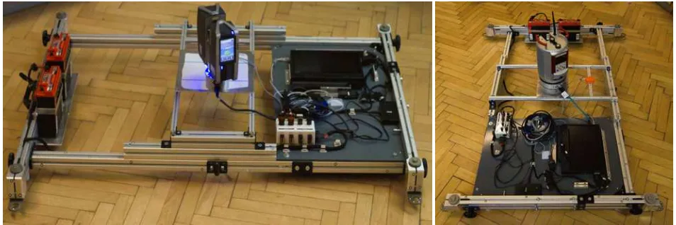
Figure 1: Left: Sensor skid, a.k.a. work-holding fixture, equipped with a FARO Focus3Dlaser scanner. Right: Skid with a Riegl VZ-400 laser scanner. Both skids are also equipped with a low-price MEMS IMU (xsens MTi).
few millimeters. Terrestrial laser scanning is the state of the art for digitalization of complex factory environments. When paired with classical surveying, terrestrial LiDAR delivers accurately referenced geo-data, which may be used for topographic pur-poses. However, many applications exist, for example as-built documentation of industrial plants and factories, ship-building, interior planning, and applications which either do not require the reference to a national grid, or do not require a reference at all.
Terrestrial Laser Scanning (TLS) is a ground based technique to measure the position and dimension of objects in three dimen-sional space using either pulsed or phase-modulated-continuous laser light. Terrestrial laser scanners use a rotating mirror and a rotating laser head to deflect the laser for measurements. Mobile laser scanning describes terrestrial data acquisition from moving platforms (e.g., boats, trains, road and off-road vehicles) and is also known as kinematic laser scanning. In the mobile scenario, the scanner operates in profiler mode, i.e., they scan a slice of the environment. 3D data is then obtained by moving the system and “unwinding” the obtained measurements.
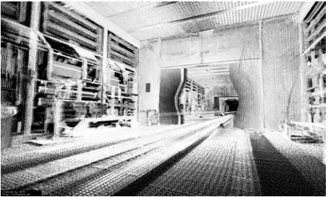
Figure 2: 3D point cloud of the entrance of a dryer tunnel ac-quired with the FARO Focus3Dscanner.
A continuously spinning terrestrial laser scanner is mounted on a skid and moved along a production line, e.g., through a drying chamber. The acquired 3D data is processed with a simultane-ous localization and mapping (SLAM) algorithm to obtain pre-cise 3D models. A detailed description of the methods can be found in Elseberg et al. (2013) and N¨uchter et al. (2010).
2 CONTINUOUS 3D SCANNING FROM A SENSORSKID
Commonly, conveyor systems are used for carrying skids and supporting products to be assembled along the assembly lines. Skid conveyors are ideally suited for automotive body shops, paint shops and final assembly operations. The base of our system con-sists of such a skid. We equipped it with a high-precision laser scanner, e.g., FARO Focus3Dor Riegl VZ-400, with electronics for connecting either of these scanners to a laptop and with a MEMS IMU (xsens MTi). Fig. 1 shows the setup.
The 3D laser scanner is configured such that the scanner spins around the vertical axis. The minimum rotation rate for the FARO scanner is 1 Hz, for the Riegl scanner it is 0.166 Hz. The field of view (vertical/horizontal) for the FARO Focus3Dis 305◦×360◦, and for the Riegl VZ-400 is 100◦×360◦. The system is cal-ibrated, i.e., the position and orientation of the sensor is deter-mined on the skid. We acquire time-stamped data while moving through the production line.
3 SEMI-RIGID OPTIMIZATION FOR SLAM
We developed an algorithm that improves the entire trajectory of the skid simultaneously. Unlike previous algorithms, e.g., by Stoyanov and Lilienthal (2009) and Bosse and Zlot (2009), it is not restricted to purely local improvements. We make no rigidity assumptions, except for the computation of the point correspon-dences. We require no explicit motion model although such infor-mation may be incorporated at no additional cost. The algorithm requires no high-level feature computation, i.e., we require only the 3D points themselves.
The motion of the mobile laser scanner between timet0andtn creates a trajectoryT ={V0, . . . ,Vn}, whereVi= (tx,i, ty,i,
tz,i, θx,i, θy,i, θz,i)is the 6 degree of freedom (DoF) pose of the skid at timetiwitht0 ≤ ti ≤ tn. Using the trajectory of the skid, a 3D representation of the environment can be obtained by “unwinding” the laser measurementsM to create the final map P. However, inaccuracies in the pose estimate which is initially computed using the known velocity estimate, as well as system-atic calibration errors degrade the accuracy of the trajectory and therefore the point cloud quality.
The current state of the art developed by Bosse and Zlot (2009) for improving overall map quality of mobile mappers in the robotics community is to coarsely discretize the time. This results in a par-tition of the trajectory into subscans that are treated rigidly. Then rigid registration algorithms like the ICP and other solutions to the SLAM problem are employed. Obviously, trajectory errors within a subscan cannot be improved in this fashion. Applying rigid pose estimation to this non-rigid problem is also problem-atic since rigid transformations can only approximate the under-lying ground truth. Consequently, overall map quality suffers as a result.
For the sensor skid a fine discretization of the time is employed, i.e., at the level of individual 2D scan slices or individual points. This results in the set of measurementsM = {m0, . . . ,mn} wheremi = (mx,i, my,i, mz,i)is a point acquired at timeti in the local coordinate system of Vi. In case Vi represents more than a single point,Vi is the local coordinate of the first point. All represented points are motion compensated with the best known interpolated trajectory. As modern laser scanners typ-ically operate at a frequency of 100–200 Hz time is discretized to 5–10 ms. Applying the pose transformation⊕we derive the pointpi = Vi⊕mi = Rθx,i,θy,i,θz,imi+ (tx,s, ty,s, tz,s)
T
in the global coordinate frame and thereby also the mapP =
{p0, . . . ,pn}. Here,Rθx,i,θy,i,θz,iis the rotation matrix that is defined by Eq. (1).
GivenM andT we find a new trajectoryT′ = {V′
1, . . . ,Vn′} with modified poses so thatPgenerated viaT′more closely re-sembles the real environment.
The complete semi-rigid registration algorithm proceeds as fol-lows: Given a trajectory estimate, we compute the point cloudP in the global coordinate system and use nearest neighbor search to establish correspondences. Then, after computing the estimates of pose differences and their respective covariances we optimize the trajectoryT. This process is iterated until convergence, i.e., until the change in the trajectory falls below a threshold.
To deal with the massive amount of data in reasonable time, we first reduce uniformly and randomly the point cloud by using only a constant number of points per volume, typically to1point per 3 cm3
. A compact octree data structure is ideally suited for this type of subsampling and for the computation of the nearest neigh-bors Elseberg et al. (2012). The octree also compresses the point cloud so it can be easily stored and processed. Furthermore, in initial stages of the algorithm, estimatesV¯i,jare only computed for a subset of posesV0,Vk,V2k, . . ., withkin the order of hundreds of milliseconds. In every iterationk is decreased so that the trajectory is optimized with a finer scale.
3.1 Pose Estimation
Our algorithm incorporates pose estimations from a rough guess of the velocity of the conveyor. Next, we use the formulation of pose estimatesV¯i,i+1that are equivalent to pose differences:
¯
Vi,i+1= ¯Vi⊖V¯j. (4)
The operator⊖is the inverse of the pose compounding operator
⊕, such thatVj=Vi⊕(Vi⊖Vj). In addition to the default pose estimates that may also be enhanced by separating all pose sensors into their own estimates as well as the proper covariances, we estimate differences between poses via the point cloudP.
Rθx,i,θy,i,θz,i =
Figure 3: Definition of the rotation matrix and the matrix decompositions.
Figure 4: Left: Before applying our semi-rigid SLAM method. Right: Correction by our semi-rigid SLAM.
minimal amount of time that must have elapsed for the laser scan-ner to have measured the same point on the surface again. To this end, we alter our search structure for finding closest points to contain time stamps as well. Points are stored in the global co-ordinate frame as defined by the estimated trajectoryT. Closest points are accepted if|pi−pj| ≤dmax. The positional error of
Here, themk,m′kis the pair of closest points in their respective local coordinate system, andNdefines a small neighborhood of points taken in the order of hundreds of milliseconds that is as-sumed to have negligible pose error. Since we will require a linear approximation of this function and⊕is decidedly non-linear we apply a Taylor expansion ofZk:
Zk(Vi,Vj)≈Zk( ¯Vi,V¯j)−
∇ViZk( ¯Vi,V¯j)∆Vi− ∇VjZk( ¯Vi,V¯j)∆Vj
.
Here,∇Virefers to the derivative with respect toVi. We create a matrix decomposition∇ViZk = MkH such that the matrix
Mkis independent ofVi. Then,Zk(Vi,Vj)is approximated as:
Zk(Vi,Vj)≈Zk( ¯Vi,V¯j)−Mk(Hi∆Vi−Hj∆Vj).
The minimum of this new linearized formulation of the error
met-ric and its covariance is given by
¯ of the independent and identically distributed errors of the error metric and is computed as
s2= (Z−MV¯i,j)T(Z−MV¯i,j)/(2M−3). (6)
The matrix decompositionMkHdepends on the parameteriza-tion of the pose compounding operaparameteriza-tion⊕. Since we employ the Euler parameterization as given in Eq. 1 the matricesMkandHi are given by Eq. (2) and (3).
3.2 Pose Optimization
We maximize the likelihood of all pose estimatesVi,jand their respective covariancesCi,jvia the Mahalanobis distance
W =X
or, with the incidence matrixHin matrix notation:
W = ( ¯V−HV)T
C−1
( ¯V−HV). (7)
following linear equation system:
(HTC−1
H)V=HTC−1¯
V. (8)
Computing the optimized trajectory is then reduced to inverting a positive definite matrix N¨uchter et al. (2010). Since a significant portion of correspondencesi, jare not considered due to the lack of point correspondences the matrix is sparse so that we make use of sparse Cholesky decomposition, Davis (2005). A consequence of this formulation is that an arbitrary poseVimust remain fixed, otherwise Eq. 8 would be under determined. This fixed pose also incidentally defines the global coordinate system. Thus, for the algorithm the optimization problem is decoupled from determi-nation of global frame coordinates of the point cloud.
4 EXPERIMENTS AND RESULTS
Experiments have been carried out with both skids from Fig. 1 at two different production lines in Wolfsburg, Germany. Fig. 2 presents an obtained point cloud. The system takes as input the approximate velocity of the skid and extracts an initial point cloud using this velocity. Afterwards, we apply our semi-rigid SLAM to correct the whole trajectory of the system. A typical trajectory consists of more than 10000 skid poses.
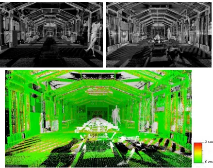
For evaluating the accuracy of the 3D data points we have also acquired a reference data set in a stop-scan-go mode. These inde-pendently acquired 3D scans have been precisely registered and form the reference model. To this reference we compare the 3D point cloud that has been captured, while the skid is in motion. To this end, both data sets are put in the same coordinate frame and point-to-point distances are calculated. Fig. 5 shows two point clouds: on the left the reference point cloud from registered ter-restrial 3D scans and in the middle the point cloud while the sen-sor skid was in motion. The rightmost part of Fig. 6 shows the deviations, i.e., for every point we compute the deviation from the ground truth model. Please note the grey parts: These are 3D points seen by the continuously rotating scanner, i.e., points on the skid, which have not been removed, and points in the envi-ronment which turn out to be occluded by terrestrial scanning at discrete poses.
Fig. 6 shows the distribution of the errors in a histogram (left) and its frequencies. 90% of the measured points have a deviation from the reference model below 2.5 cm. 3D points closer to the scanner have usually even higher precision, as scanning is done in a spherical way.
5 COLLISION DETECTION
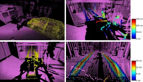
After acquiring a consistent 3D point cloud of the environment, we check whether a model moving through the environment col-lides with it, which points in the environment collide and how deep they penetrate the model. To this end we move a point cloud of the model through the point cloud of the environment along a given trajectory. Fig. 7 shows on the upper left the point cloud of the environment in magenta and the point cloud of the model in yellow. The point cloud of the model can either be acquired by measurements with a laser scanner or by sampling the surface area of a given CAD model. The given model represents a Volk-swagen Golf scaled to a width of about 3 m to make it collide with the factory environment.
Any point of the environment that is found to be closer than a radiusrto any point of the model at any point of the trajectory is classified as “colliding”. All points of the environment which are
never found to fulfill this criteria are classified as “non-colliding”. Fig. 7 shows on the lower left the colliding point cloud in yel-low and the non-colliding point cloud in magenta when moving the car model from the right figure through the environment on a straight trajectory along the assembly line. Bigger radii ofr al-low to implement “safety distances” for objects moving through the environment. In this example, we chose a radiusrof 10 [cm].
After the point cloud of the environment has been partitioned in colliding and non-colliding points, we calculate for all colliding points an estimate of their maximum depth of penetration into the model along its path. For each colliding point we find the clos-est non-colliding point in the environment and take their distance as a heuristic for the depth of penetration. This heuristic works well for the common cases of objects protruding the volume of an assembly line. Fig. 7 shows in the right column the color-coded depth of penetration.
Computation of points within a radiusrfor the collision detection and of the closest non-colliding points in the environment for cal-culating the penetration depth are done by creating and searching in ak-d tree of the environment. Using this data structure, every lookup can be done inO(log (n))time withnbeing the num-ber of points in the environment. Therefore, collision detection can be done inO(lmlog (n))time withmbeing the number of points in the model andlbeing the number of points in the tra-jectory. The number of points in the environmentnis reduced by only considering those points within a bounding sphere of the model. The number of points in the model can only be reduced until points which are neighbors on a surface are a maximum dis-tance ofrapart from each other. Using a model of 10000 points, moved through an environment of over 840000 points on a trajec-tory with 1000 poses (as seen in Fig. 7), collision detection takes about 11 seconds and depth of penetration calculation about 2 seconds on a single threaded desktop machine.
6 SUMMERY, CONCLUSION, AND FUTURE WORK
This paper has presented the essentials of a novel system for pre-cise 3D modeling of production lines. With the built sensor skid we can access and digitize areas which are hard to inspect other-wise. We showed the ability to calculate the application specific depth-of-penetration.
Needless to say a lot of work remains to be done. In future work, we will concentrate on putting the acquired data into a global frame of reference, i.e., geo-referencing, on clustering the collid-ing point cloud, and on applycollid-ing a divide-and-conquer methods to cope with longer trajectories. Currently, 100 6D poses are gener-ated per second, which implies that the linear system of equations for solving our SLAM problem contains 600 entries per second.
References
Bosse, M. and Zlot, R., 2009. Continuous 3D Scan-Matching with a Spinning 2D Laser. In: Proceedings of the IEEE Inter-national Conference on Robotics and Automation (ICRA ’09), pp. 4312–4319.
Davis, T. A., 2005. Algorithm 849: A Concise Sparse Cholesky Factorization Package. ACM Trans. Math. Softw. 31(4), pp. 587 – 591.
0 cm 5 cm
Figure 5: Above left: 3D Point Cloud acquired in a stop-scan-and-go fashion. Above right: Point Cloud acquired in continuous motion. Below: Derivation of the two point clouds in a centimeter scale.
0 50000 100000 150000 200000 250000 300000 350000 400000 450000
0 1 2 3 4 5
deviation [cm]
N
u
m
b
er
o
f
m
ea
su
re
m
en
ts
0 0.1 0.2 0.3 0.4 0.5 0.6 0.7 0.8 0.9 1
0 0.5 1 1.5 2 2.5 3 3.5 4 4.5 5
deviation [cm] frequency fraction of points with error< x
Figure 7: Upper Left: a view of two point clouds (environment and car). Lower Left: two separated point clouds (non-colliding and colliding points). Right Column: Color-coded depths of penetration
Elseberg, J., Magnenat, S., Siegwart, R. and N¨uchter, A., 2012. Comparison of Nearest-Neighbor-Search Strategies and Im-plementations for Efficient Shape Registration. Journal of Software Engineering for Robotics (JOSER) 3(1), pp. 2 – 12.
N¨uchter, A., Elseberg, J., Schneider, P. and Paulus, D., 2010. Study of Parameterizations for the Rigid Body Transforma-tions of The Scan Registration Problem. Journal Computer Vision and Image Understanding (CVIU) 114(8), pp. 963–980.