www.elsevier.com/locate/spa
A possible denition of a stationary tangent
U. Keich
Mathematics Department, University of California, Riverside, CA 92521, USA
Received 25 February 1998; received in revised form 22 November 1999; accepted 2 December 1999
Abstract
This paper oers a way to construct a locally optimal stationary approximation for a non-stationary Gaussian process. In cases where this construction leads to a unique non-stationary ap-proximation we call it a stationary tangent. This is the case with Gaussian processes governed by smoothn-dimensional correlations. We associate these correlations with equivalence classes of curves in Rn. These are described in terms of “curvatures” (closely related to the classical curvature functions); they are constant if and only if the correlation is stationary. Thus, the stationary tangent, att=t0, to a smooth correlation, curve or process, is the one with the same curvatures at t0 (but constant). We show that the curvatures measure the quality of a local stationary approximation and that the tangent is optimal in this regard. These results extend to the smooth innite-dimensional case although, since the equivalence between correlations and curvatures breaks down in the innite-dimensional setting, we cannot, in general, single out a unique tangent. The question of existence and uniqueness of a stationary process with given curvatures is intimately related with the classical moment problem and is studied here by using tools from operator theory. In particular, we nd that there always exists an optimal Gaussian approximation (dened via the curvatures). Finally, by way of discretizing we introduce the notion of -curvatures designed to address non-smooth correlations. c 2000 Elsevier Science B.V. All rights reserved.
MSC:60G10; 60G15; 34G10; 47A57
Keywords: Stationary processes; Curvature functions; Stationary tangent; Moment problem; Tri-diagonal matrices
1. Introduction
Stationary processes have been thoroughly studied and a comprehensive mathematical theory has been developed based primarily on the spectral distribution function. As a natural extension people considered “locally stationary processes”. Intuitively, these are non-stationary processes that on a suciently small time scale do not deviate considerably from stationarity. To mention just a couple of approaches: Priestley has studied this problem through what he denes as the evolutionary spectrum (Priestley, 1988, p. 148) and later he (Priestley, 1996), and independently Mallat et al. (1998)
E-mail address:[email protected] (U. Keich)
looked at the problem from wavelets point of view. These authors base their work on an analysis of the (real) correlation function. Such common practice can be justied, for example, by considering zero-mean real Gaussian processes which are studied in this paper as well.
The related question that we consider here was suggested to us by McKean: can one dene a “stationary tangent” for a non-stationary Gaussian process? The linear tangent, at t0, to a function f, is the best local linear approximation to f at t0. One can
compute it from f′(t0), provided the function is dierentiable. Similarly, the stationary
tangent dened in this paper is an optimal stationary approximation to a suciently smooth non-stationary, say, correlation. Consider the following example. The correlation
R(t; s) = cos(!(t)−!(s)), is stationary if and only if ! is a linear function of t, but
is the stationary tangent to R at t0, and it is indeed so according to our denition.
We say that the stationary process ˆX is an optimal stationary approximation to the process X at t0, if it sequentially minimizes E|X(t0k)−Xˆ
(k) t0 |
2 for k= 0;1;2: : : More
precisely, consider the following decreasing sets of processes:
A0
Then, ˆX is an optimal stationary approximation if ˆX∈T
nAn. We show that ˜X, our stationary tangent to X at t0, is such an optimal approximation (Theorem 4). In some
cases it is the unique such optimal approximation. Since E|X(t0k)−Xˆ
t0 a.s., the optimal stationary
approximation is also an approximation of optimal order in the a.s. sense. This raises the question of, what we term, the order of stationarity ofX at t0. It is dened as the
maximal dfor which |Xt−Xˆt|=O(t−t0)d+1 a.s. We show that the same mechanism
that allows us to dene the stationary tangent can also be used to determine the order of stationarity. We next provide a rough outline of this mechanism.
Throughout this paper we consider three related (smooth) objects: a 0-mean real Gaussian process, X, a correlation function, R, and a curve x (in Rn or l2), which we associate with R via R(t; s) =hxt;xsi. The main idea is to associate “curvatures” to our equivalence classes of curves, and thereby to the corresponding correlations and processes. These curvatures are positive functions closely related to the classical curvature functions and, as explained next, are well suited for the problem of stationary approximations. Indeed, stationary objects have constant curvatures which yields, in principle, a way to dene a stationary tangent. For example, the stationary tangent correlation att0 to the correlation R, is the one which itsconstant curvatures are equal
to the curvatures ofRatt0. For processes, the denition of the tangent is slightly more
In describing the tangent correlation we implicitly assumed that the curvatures of
R at t0 uniquely determine a stationary correlation. However, this is only assured to
be the case if the associated curve is in Rn, a case which is studied in Section 2 of this paper. More generally, while the curvatures approach will always yield an optimal stationary approximation, it might not yield a unique such approximation. As we show, the question of reconstructing a stationary tangent from its constant curvatures is equiv-alent to Stieltjes’ moment problem (Section 3.3 explains more about the connection with the moment problem).
Using results from the theory of evolution equation in a Hilbert space and of self-adjoint extensions of symmetric operators, we study in Section 3.2 the general case of constant curvatures. In particular, we settle the aforementioned question of existence and uniqueness of an optimal stationary approximation, which in the case of non-uniqueness, we call a curvature stationary approximation. Note that an “n -dimensional” correlation (i.e., the associated curve is in Rn) is stationary if and only if its curvatures are constant. However, for general curves in‘2, the correlation might not be stationary even though its curvatures are constant (Claim 3.8).
Finally, since the curvatures of any stationary process Xhave vanishing derivatives, the aforementioned order of stationarity depends on, roughly, how many derivatives of the curvature functions ofX vanish at t0. Thus, we can readily determine the order of
stationarity of X from the derivatives of the curvatures. Naturally, the tangent, being optimal, is a stationary approximation of this order. Similarly, we dene and treat the order of stationarity of a correlation and a curve.
In a following paper we will show how the curvature scheme can be extended to non-smooth correlations, as well as to non-instantaneous stationary approximations. The basic idea, as presented here in Section 4, is to use nite dierences instead of derivatives.
2. Stationary tangents in the nite-dimensional setting
2.1. Correlation, curves and curvatures
Any correlationR of a mean-square continuous Gaussian process dened on a com-pact time interval I, can be expressed, by Mercer’s theorem, as
R(t; s) =
∞
X
i=1
iei(t)ei(s);
wherei¿0 are the eigenvalues and ei’s are the eigenvectors of the integral operator dened by the kernel R. Thus, with xi(t)=d √iei(t),
R(t; s) =
∞
X
i=1
xi(t)xi(s): (1)
Denition.
• A correlation R is n-dimensional if the sum in (1) extends up to n and if the xi’s are linearly independent.
• A Gaussian process is n-dimensional if its correlation is such.
We dene an equivalence relation on (continuous) curves xt d
= [x1(t); x2(t); : : : ;
xn(t)] ∈ Rn as follows: The curves x and y are considered equivalent, if there ex-ists a xed orthogonal transformation of Rn; U such that y=Ux. Let [x] denote the equivalence class of x. Then we can associate an n dimensional correlation with [x] via R(t; s)=dhxt;xsi, where h;i is the standard inner-product in Rn. Conversely, given
R, (1) yields a corresponding curve, and we nd
Claim 2.1. There is a 1 : 1 onto correspondence between continuous correlations of dimension 6n;and equivalence classes of (continuous) curves in Rn.
Proof. Since orthogonal transformations preserve the inner-product, for any y ∈[x]; R(t; s)=hyt;ysi, hence the correspondence is well dened on our equivalence classes and from (1) we learn it is onto. As for 1:1, suppose that for allt; s∈I; hxt;xsi=hyt;ysi. In particular it follows that if xt=xs then yt=ys. Hence Uxt7→yt is a well dened map between the traces of the two curves. Furthermore, U can be extended uniquely to an orthogonal map between the subspaces generated by the traces of the curves. In particular it can be extended as an orthogonal map of Rn, and hence y∈[x].
In this geometric context, stationary correlations have a distinctive property; since
R(0) =hxt;xti the curve obviously lies on a sphere in Rn, and fort; t+r∈I,
xt
|xt|
; xt+r |xt+r|
=R(r)
R(0);
is independent of t. Hence the curves that are associated with stationary correlations are angle preserving, or (borrowing Krein’s terminology (Krein, 1944)) helical curves on a sphere in Rn.
Next we introduce a variant of the classical curvature functions, but in order to do so we need to restrict attention to:
Denition 2.2. A curve x∈RN is s.n.d, or strongly n dimensional (N¿n), if it isn
times continuously dierentiable, and for eacht∈I,{xt(k)}nk−=01 are linearly independent,
while {x(tk)}nk=0 are dependent.
Remark. If [x] = [y], then clearly x is s.n.d if and only if y is. Therefore we can talk about s.n.d correlations as well. Later, Denition 2.10 will specify this in terms of R
itself.
Letx∈Rn be s.n.d, and let{C
i(t)}ni=0−1 be the result of the Gram–Schmidt procedure
Denition 2.3.
• The ithcurvature function of x is i=dhC˙i−1;Cii:
• The orthogonal frame of x at time t is the n×n matrix Vt whose rows are Ci(t). • The curvature matrix of x is the n×n skew-symmetric tridiagonal matrix valued
function Kt withKt(i; i+ 1) =i(t) for i= 1; : : : ; n−1.
Remark. The classical curvature functions can be dened in an analogous way; to get those, apply the Gram–Schmidt procedure to{x(ti):i= 1; : : : ; n} (see e.g. Spivak, 1979). The reason for introducing our variant of the curvatures is that the classical curvatures are invariant under Euclidean transformation of Rn, while our equivalence classes of curves are determined up to orthogonal transformations.
The dynamics of the orthogonal frame (called the Frenet frame in the classical version) is described by:
Claim 2.4. For i= 1;2; : : : ; n−1; i(t)¿0 and ˙
V =KV: (2)
Proof. Since theCi’s are orthonormal it follows thathC˙i;Cji=−hCi;C˙ji, hence (2) holds
with a skew-symmetric matrix K. Since
Span{x;x(1);x(2); : : : ;x(k−1)}= Span{C0;C1; : : : ;Ck−1};
it is obvious thathC˙i;Cji=0 forj¿i+2, henceK is tridiagonal. Finally by our denition of the Gram–Schmidt process, hx(i);C
ii¿0 hence i=hC˙i−1;Cii¿0.
We show next that with one more curvature function, 0 d
=|x|, the curvatures char-acterize the equivalence classes of s.n.d curves, and therefore s.n.d. correlations.
Note that if we dene k= 0 ford k6∈ {0; : : : ; n−1}, then (2) can be rewritten as
˙
Ck=−kCk−1+k+1Ck+1; k= 0; : : : ; n−1: (3)
Repeatedly dierentiating the equation x=0C0 while using (3) yields
x=0C0;
˙
x= ˙0C0+01C1;
x= ( 0−012)C0+ (2 ˙01+0˙1)C1+012C2:
..
. (4)
More generally,
Claim 2.5. With x(k)=Pk
i=0ckiCi (by induction on k) we have:
• cki are polynomials in{(lj): 06l6k ;06j6k−l}.
• ck
k=01: : : k; and k does not appear in cki for i ¡ k.
• Ifk¿n this representation still holds (i.e.; thecki are the same polynomials as for
Claim 2.6. Letxbe an s.n.d curve. It denes n positive curvature functions{i(t)}ni=0−1;
such that; i isn−i times continuously dierentiable;and these curvatures are shared by any curve which is equivalent to x.
Proof. As stated in Claim 2.5,hx(i);Cii=01: : : i. Note that the left-hand side is the
class, they dene the same curvatures.
Note that2i is the determinant of the Grammian matrix dened byx;x(1);x(2); : : :x(i):
Suppose now that you are given the curvatures, or rather:
Denition 2.7. A curvaturetype matrix is a tridiagonal skew-symmetric matrixK with
K(i; i+ 1)¿0.
Claim 2.8. Let U be an orthogonal matrix and let Kt be a curvature type matrix valued function such that i
d
=Kt(i; i+ 1) is n−i times continuously dierentiable. Then; there exists a unique s.n.d curve x∈Rn such that; Kt is the curvature matrix of x at time t and U is its orthogonal frame att= 0.
Proof. Let Vt be the unique solution of (2) with V0=U, and dene xt=0(t)Vt∗e1.
Then, x is an n times continuously dierentiable curve inRn (here we use the corre-sponding dierentiability of the curvatures). Note thatVt is an orthogonal matrix since
Kt is skew symmetric. It is not hard to see that the result of Gram–Schmidt applied to
{x(tk)}kn−=01 is{Ci(t)} n−1
of x. Finally, if yis another such s.n.d curve then, with Wt being its orthogonal frame, ˙
W =KW and W0=U. Therefore, by the uniqueness of V; W ≡V and y≡x.
Claim 2.9. Let {i}ni=0−1 be n positive(curvature) functions withi being n−i times continuously dierentiable. There exists a unique (up to equivalence) s.n.d curve;
x∈Rn; with these curvatures.
Proof. Letx andy be two curves which share these curvatures. According to the pre-vious claim, these are uniquely dened given their frames att= 0; Vx(0), respectively,
Vy(0). Let U uniqueness part of the previous claim that w ≡y. That is, x and y are in the same equivalence class.
where all the derivatives are evaluated at (t; t). Using the above identity in (6) yields the curvatures in terms of R directly. Furthermore Denition 2.2 can now be phrased in terms of R.
Denition 2.10. A correlation R is s.n.d if its derivatives @i t@
j
sR, max{i; j}6n, exist (and are continuous), and if for each t∈I, Dn−1(t)¿0, while Dn≡0.
Remark. SupposeR(t; s) =hxt;xsi. One can verify using (7) thatR is s.n.d if and only if x is such. Since we give a similar proof for the innite-dimensional case in Claim 3.1, we omit it here.
The following claim is now an immediate consequence.
Claim 2.11. There is a1 : 1 correspondence between:
• s.n.d correlations;
• equivalence classes of s.n.d curves;
• n positive curvature functions 0; : : : ; n−1; where i is in Cn−i(I).
Remark 2.12.
• Suppose thatx∈Rn is a smooth curve {xt(i)}ni=0−1 is linearly independent for all t∈
I except for a nite number of points. Then one can readily dene the curvatures of this curve. The problem is that now there might be non-equivalent curves with the same curvatures. Consider for example the 1-dimensional curves xt= (t3) and
˜
xt= (|t|3). These are non-equivalent curves, yet their curvatures, 0(t) = ˜0(t) =|t|3
and 1 ≡˜1 ≡ 0 are identical. The fact that ˜x is not entirely smooth at t= 0 is
irrelevant to the phenomenon; there is indeed a discontinuity in the orthogonal frame, but it is not reected in the curve itself.
2.2. Curvatures and stationary correlations
The next theorem is the motivation behind the introduction of the curvatures.
Theorem 1. The curvatures are constant if and only if the s.n.d correlation is stationary.
Remark. In particular anyn dimensional stationary correlation is an s.n.d one. In view of that we will be omitting the acronym s.n.d where there is no room for confusion.
Proof. It follows immediately from (6) and (7) that if the correlation is stationary, then the curvatures are constant. On the other hand, if the curvatures are constant (2) is explicitly solvable: Vt= etKV0. We can assume V0=I and since xt =0(t)Vt∗e1
always holds, we get
xt=0e−tKe1:
In particular
R(t; s) =h0e−tKe1; 0e−sKe1i=20he1;e(t−s)Ke1i;
which is obviously a stationary correlation.
In proving the last theorem we found that, in the stationary case,R(r)=2
0herKe1;e1i.
Using the spectral resolution for the skew-symmetric K, K=P
j i!juj⊗uj (where
±i!j are the eigenvalues anduj are the eigenvectors), we nd
R(r) =02
*
exp X j
ir!juj⊗uj !
e1;e1
+
=02X
j
eir!j|uj(1)|2: (8)
This identies the spectral distribution function of R as the spectral measure of the Hermitian matrix iK obtained from the generating vector e1. In fact it is the same as
the spectral measure of the real, symmetric matrix, ˆK, obtained fromK by ipping the signs of the elements in the lower sub-diagonal:
Claim 2.14. If A is a real skew-symmetric tridiagonal matrix; then iA and Aˆ are unitary equivalent matrices. Moreover; their spectral measures with respect to e1 are
identical.
Proof. Let U be the diagonal unitary matrix with U(j; j) = ij, then U(iA)U−1= ˆA.
In other words, iA is the same as ˆA represented by the basis {ije
j}. Since e1 is an
eigenvector of U, the corresponding spectral measures are identical.
Going back to (8), we notice that since K is real, the eigenvalues i!j come in conjugate pairs, as do the corresponding eigenvectors uj. Thus, with m= [(n+ 1)=2],
R(r) =20 m X
j=1
2
jcos(!jr);
where 2
j = 2|uj(1)|2, except if n is odd, in which case !1= 0 is an eigenvalue and
21=|u1(1)|2. This shows that, assuming smoothness, a nite dimensional stationary
correlation is necessarily of the type just mentioned (i.e., the spectral distribution func-tion is discrete with n+ 1 jumps). One can show that is also the case without assuming smoothness, which is then a corollary (see von Neumann and Schoenberg, 1941). In terms of the paths, we have the following geometric interpretation: any angle preserv-ing (helical) curve on a nite dimensional sphere is equivalent to a bunch of circular motions, of radii i and angular velocities!i, performed in orthogonal planes.
Finally a word of caution. So far we discussed nite dimensional processes dened on a nite time interval. In the stationary case, if one wants to talk about the spectral distribution function, then tacitly it is assumed that there is one and only one way to extend the given stationary correlation to the whole line. In Krein (1940) shows you can always extend a positive-denite function (or a correlation of a stationary process) to the whole line, retaining its positive-denite character. This extension might be unique, as is the case for the nite dimensional correlations we are dealing with here.
2.3. Tangents
Theorem 1 allows us to introduce various notions of tangent, all based on the idea of freezing the curvatures. There are three objects which are of interest here: the correlation, the curve, and the process itself. For each of these we will dene its stationary tangent and then justify the terminology.
Proof. LetR be an s.n.d correlation, itsstationary tangentat (t0; t0), is the correlation
dened by the (constant) curvatures 0(t0); : : : ; n−1(t0).
Remark.
• If R is stationary, then its tangent at t0 is itself.
• LetRbe an s.n.d correlation, then given all its tangents ˜Rt0,t0 ∈I, we can reconstruct
Denition. Let x be an s.n.d curve in Rn and let K be its curvature matrix, and V
its orthogonal frame. Thestationary tangent curve tox at t0 is the stationary curve ˜x
dened by
• The curvature matrix of ˜x is ˜K ≡Kt0.
• The orthogonal frame of ˜x at t=t0 is Vt0.
Remark.
• By Claim 2.8, there exists a unique tangent curve, furthermore, ˜
xt=0(t0)[exp((t−t0)Kt0)Vt0]∗e1:
• The denition of the tangent curve and the last equation hold also for an s.n.d curve
x∈RN with N ¿ n (cf. Remark 2.12).
• If x is stationary, then ˜x≡x (Claim 2.8 again).
• If ˜x is the tangent curve to x at t0, then ˜R(t; s) =hx˜t;x˜si is the tangent correlation toR at (t0; t0).
Finally, we dene the tangent process. Let X be an s.n.d Gaussian process, i.e., it has an s.n.d correlation R. Then, there exists an n dimensional Gaussian vector,
= [1; 2; : : : ; n] (where i are independent N(0;1) random variables), and an s.n.d curve, xt, such that,
Xt=h;xti=
n X
i=1
ixi(t): (9)
Remark. The Karhunen–Loeve expansion is an example of such a representation: with
R(t; s) =Pn
i=1 iei(t)ei(s) (spectral decomposition of R), one denes i d
=R
I Xtei(t) dt (Loeve, 1963), and we add xi(t)
d
=√iei(t).
Denition 2.15. The stationary tangent process at t0 is ˜Xt d
=h;x˜ti where ˜x is the stationary tangent curve to x at t0.
Remark 2.16.
• The representation X=h;xi where i are N(0;1) independent random variables is not unique. However, if X=h;xi=h;yi, where i are also independent and N(0;1), thenR(t; s) =hxt;xsi=hyt;ysi, sox=Uy for some xed orthogonalU and it follows that=U. Thus the tangent process is well-dened.
• X˜ is a stationary process and it is jointly Gaussian with X, meaning that any linear combination,
X
i
iXti+ X
j
jX˜tj; i; j∈R;
is a Gaussian random variable.
• The correlation of ˜X is the tangent correlation att0 (in particular, it is s.n.d).
• Since the map T :Rn →L2(dP), described by Tx
t=d Xt=h;xti, is a well-dened isometry, Gram–Schmidting X(tk) is equivalent to Gram–Schmidting x
(k)
t . Thus, for each t, there exist n independent N(0;1) random variables, Vk(t)
d
=T(vk(t)), such that, with ck
i as in Claim 2.5,
X(tk)= k X
i=0
ckiVk(t):
This yields another way to describe the tangent process:
˜
Xt=ht;x˜ti=0(t0)[V0(t0);V1(t0); : : : ;Vn−1(t0)] exp(−(t−t0)Kt0)e1:
Note that to nd Vk(t0) from Xt(k), we need “only” to compute cik, which can be done directly from the correlation R.
So far we gave some justication for the usage of the term “stationary tangent”. However, the most important one is that, as we will see in the next section, the tangent provide us with an optimal stationary approximation. Before we get there, let us take another look at the example from the introduction.
Example 2.17. The stationary tangent at t0 to:
• the correlation R(t; s) = cos(!(t)−!(s)) is, ˜
R(t; s) = cos( ˙!(t0)(t−s)):
• the curve xt= [cos(!(t));sin(!(t))] is ˜
xt= [cos(!(t0) + ˙!(t0)(t−t0));sin(!(t0) + ˙!(t0)(t−t0))]:
• the process: Xt=cos(!t) +sin(!t), where and are independent N(0;1), is ˜
Xt=cos(!(t0) + ˙!(t0)(t−t0)) +sin(!(t0) + ˙!(t0)(t−t0)):
This simple example agrees with our intuition. There are examples of non-trivial tangents, as we shall see later on.
2.4. Curvatures and stationary approximations
This section explains why the curvatures are well adapted for the study of local stationary approximations.
Let x and x be strongly n=n dimensional curves in RN with corresponding frames and curvatures,Ci=Ci, respectively, i=i. Then,
Claim 2.18.
x(t0k)= x (k)
t0 fork= 0; : : : ; m (10)
if and only if
(kp)(t0) = (kp)(t0) and Ck(t0) = Ck(t0)
Proof. By Claim 2.5, (10) follows immediately from (11). Conversely, if (10) holds, then obviously Ck(t0) = Ck(t0) for k= 0; : : : ; m (hence if m¿n, necessarily n= n). Let Nk(t)=dhxt(k);xt(k)i. Then, (10) implies that Nk(p)(t0) = N
(p)
k (t0) for k +p6m.
A somewhat technical argument, which is postponed to Claim 5.2, now shows that
k(p)(t0) = k(p)(t0) fork+p6m.
In view of the last claim and the fact that stationary curves have constant curvatures, we dene
Denition 2.19. The order of stationarity at t0 of an s.n.d curve, x, is
d(t0) d
= min{m:(kp)(t0)6= 0 withk6m−1;16p6m−k} −1:
Note that if x is stationary, then d≡ ∞. The following theorem is an immediate corollary of the last claim. Let x be an s.n.d curve with d=d d(t0)¡∞, then
Theorem 2a. About t=t0; xˆ is a stationary; local approximation to x; of optimal
order; if and only if
ˆ
i≡i(t0) and vˆi(t0) =vi(t0) fori= 0; : : : ; d:
In this case;kxˆt−xtk= O(|t−t0|d+1)butO(|t−t0|d+2) fails. In particular; the tangent
curve is a stationary approximation of optimal order.
As for processes, let X and ˆX be strongly n=nˆ dimensional Gaussian processes which are jointly Gaussian. Then, Xt=h;xti and ˆXt =h;xˆti where is a vector of independent N(0;1) random variables and x and ˆx are s.n.d curves in RN, where
N¿max(n;nˆ). We can use
E|Xt−Xˆt|2=kxt−xˆtk2;
as a measurement of the quality of the approximation. An immediate corollary is that, about t=t0; Xˆ =h;xˆi is a stationary local approximation of optimal order to the
process X, if and only if ˆx is an approximation of optimal order to x at t=t0. Thus,
Theorem 2a has an exact analogue in terms of processes (with Vk from Remark 2.16 replacing vk). However, since X and ˆX are jointly Gaussian,
Prob{|Xt−Xˆt|= O(|t−t0|k+1)}¿
⇔Var(X(t0j)−Xˆ (j)
t0 ) = 0 j6k
⇔ kx(t0j)−xˆ (j) t0 k
2= 0 j6k:
Thus, we get the bonus in terms of almost sure properties as stated in the following theorem. Let d=d(t0) be as in Denition 2.19, then
Theorem 2b.
• If at t=t0; Xˆ is a stationary approximation of optimal order; then
ˆ
and
|Xˆt−Xt|= O(|t−t0|d+1) a:s:
• The tangent process is an optimal stationary approximation.
• For any stationary process; Xˆ; jointly Gaussian with X;
Prob{|Xt−Xˆt|= O(|t−t0|d+2)}= 0:
To prove the analogous result for correlations we need the following claim, the proof of which is postponed to Section 5. In what follows, R is an s.n.d correlation.
Claim 2.20. There is a perfect equivalence between {@kR|
(t0; t0): k6n} and
{(kp)(t0): 06k6[n=2];06p6n−2k}.
Denition 2.21. The order of stationarity of R at (t0; t0) is dened as
d(t0) d
= min{2k+p:p¿1; k¿0; k(p)(t0)6= 0} −1:
Let the stationary order of R at t0 be d=d(t0)¡∞, then
Theorem 3. About the point(t0; t0); Rˆ is a stationary local approximation;of optimal
order;to the correlationR;if and only ifˆi≡i(t0)fori=0;1; : : : ;[d=2].In particular;
the stationary tangent correlation is such. For any optimal order approximation; |S(t; s)−R(t; s)|= O(d+1) but |S−R| 6= O(d+2) (where =p
(t−t0)2+ (s−t0)2).
Proof. Let R and ˆR be two smooth correlations. By Claim 2.20, |R−Rˆ|= O(n+1),
about the point (t0; t0), if and only if
(kp)(t0) = ˆ(kp)(t0) for 06k6[n=2]; 06p6n−2k: (12)
If ˆRis stationary, then ˆ(kp)=0 forp¿1. Hence, (12) holds, if and only ifk(t0)= ˆk(t0)
for 06k6[n=2], and (kp)= 0 for 06k6[n=2], 16p6n−2k. Since the latter can only hold if n6d, it follows that d+ 1 is the optimal order for any stationary local approximation ofR. Moreover, it is clear that the stationary tangent attains this optimal order.
Remark. A variant of the previous theorems is obtained by assuming{i(t): i6m−1} are constant in an intervalI. In this case, for anyt0∈I, the stationary tangent att0 will
yield |R−St0|= O(
2m+1) for correlations, and O(|t−t
0|m) for curves and processes.
Furthermore, ifm(t) is not constant in I, then this is the best we can do, in the sense that there will be points t0∈I for which the next order of approximation fails.
minimizers in a sense that is made precise as follows: Let ˜x be the stationary tangent
the analogous result for processes. This proves that the tangent is indeed an optimal stationary approximation as dened in the introduction.
Proof of Theorem 4. (13) follows trivially from (14). For the other implication we use induction on k. Fork= 0, kx˜t0−xt0k= 0, so obviously (13) implies ˆxt0=0(t0)Ct0
and (14) holds. Assume by way of induction that (14) holds for k −1. Then, by Claim 2.5,
which completes the induction. As for (15), the same induction should work: just start it with k=−1, and note that since
k˜0˜1: : :˜kC˜k(t0)−0(t0)1(t0): : : k(t0)Ck(t0)k2= 0;
(15) follows.
Let x be an s.n.d curve of stationary degree d ¡∞ and let ˜x be its tangent curve, at t0. From the last theorem and Theorem 2a, we can deduce:
Claim 2.22. For any stationary curve xˆ;
0¡lim
Remarks.
• ReplacingE|Xt|2 with kxtk2, etc., we get the analogous result for processes.
• The analogue for correlations is false. For example, it is possible that with ˜R the tangent to a correlation R, of degree 1, there exists a stationary correlation ˆR, with
∞¿ lim
where ˆR is a stationary correlation and ’ is a smooth real function. Note that Exam-ple 2.17 is a special case of this one. The corresponding curves are following along stationary paths, where the timing is dictated by ’(t). One can check that for these correlations, i(t) = ˙’(t) ˆi for i¿1 and that 0≡ˆ0. Therefore,
Intuitively, the stationary tangent should be
Rt0(t−s)≈
curvatures vanish. Therefore, the curvature tangent is of the form
˜
Rt0(t−s) =1(t0) 2cos[!
1(t0)(t−s)] +2(t0)2cos[!2(t0)(t−s)]; (16)
where!i(t0) (i= 1;2) are the eigenvalues of the symmetrized curvature matrix ˆK(t0)
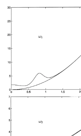
(Claim 2.14). Computing these explicitly we nd
!1(t0) = 3t20+ O(t− 6
0 ); !2(t0) = 2t0+ O(t0−5):
The weights i are somewhat harder to get explicitly, so you are invited to inspect a numerical representation in Figs. 1 and 2. Note that there is a fast convergence to the tangent we anticipated intuitively. The reason the curvature tangent does not resemble our intuition fort61:5 is related to the fact that the change in the intuitive “stationary frequency” is big relative to the frequency itself. Also at t= 0 there is a violation of the “strong 4 dimensionality”. Since 1= 12
√
18t4+ 8t2, the degree of stationarity of
this correlation is d= 1.
Example 2.25.
R(t; s) =1
2cos[cos(t)−cos(s)] + 1
Fig. 1. Example 2.24: frequencies of the curvature tangent. The eigenvalues,!(t0), of the “symmetrized” curvature matrix, ˆK(t0), ofR(t; s) =12cos(t2−s2) +1
2cos(t
3−s4). The rst one is compared with 3t2while the second with 2t. See Fig. 2 for the corresponding weights.
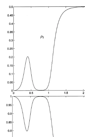
Here we nd
0≡1; 1≡ √12; 2=√12
p
4 cos4t−4 cos2t+ 3; 3¿0:
Intuitively we expect the stationary tangent to be ˜
Rt0(t−s)≈ 1
2cos[sin(t0)(t−s)] + 1
Fig. 2. Example 2.24: radii of the curvature tangent. The weights,(t0), of the spectral function associated with the curvature matrixK(t0) from the previous gure.
The stationary correlation at the right-hand side, S, matches 0, and 1, but fails with
2(t0). Thus
|R(t; s)−S(t−s)|= O(4):
The curvature tangent matches2(t0) and so
Note thatRis=2 periodic in t ands, and at the lattice points (i=2; j=2), its (strong)
dimension is not 4. The theory developed so far can be readily extended to this kind of isolated points, where the dimension suddenly drops. It should be pointed out, that in this example, the accuracy of the curvature tangent at these points is better than at the regular points. As for how this tangent correlation looks: it is again of the form (16). The frequencies and radii (which are found from the spectrum of ˆK) are depicted in Figs. 3 and 4.
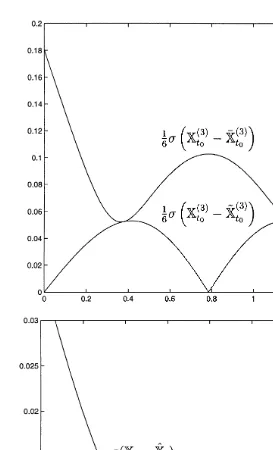
Finally, the stationary degree of the corresponding curve=process is 2, while the naive approach will only match one derivative. The lower diagram of Fig. 5 compares the standard deviation of the errors these two stationary aproximations generate. Both the tangent and the intuitive approximation are dened at t0 ==8. To demonstrate
Theorem 4, the upper diagram of Fig. 5 compares the graphs of h16X(3)t0 − 1 6X˜
(3) t0
i
andh1 6X
(3) t0 −
1 6X
(3) t0
i
, where X is a stationary process that agress with the rst three curvatures of X att0 but 3= 1:25 throughout. The graphs meet at the two points,t0,
where 3(t0) = 1:25. It happens that ′2(=4) = 0, and by Theorem 2b, the degree of
stationarity jumps to 3 at this point. This is reected in hX(3)=4−X˜(3) =4
i
= 0, as you can check in the graph.
3. The smooth innite-dimensional case
3.1. The curvatures and the problems
Only part of the theory just developed for then-dimensional case holds in the smooth innite-dimensional case. As in Section 2.1, we can associate innite-dimensional, con-tinuous correlations, dened on I ×I, with equivalence classes of continuous paths dened on I. The only dierence is that the paths are in l2 now, so the sum (1)
is innite; the equivalence is up to an isometry of the space. Claim 2.1 holds with essentially the same proof.
As in the nite-dimensional case, we are interested in a subclass of correlations and paths, to which we can assign curvatures.
Denition.
• A curve x is s.i.d if for any ’∈l2,hx
t;’i is aC∞ (real) function and if, for any
t∈I,{xt(k):k∈N} is a linearly independent set in l2.
• A correlationRis strongly innite dimensional (s.i.d) if it is innitely dierentiable, and for all i∈N andt∈I; Di(t)¿0 (where Di is dened as in (7)).
The next claim assures us that these two objects should indeed share the same title.
Claim 3.1. Suppose R(t; s) =hxt;xsifor all t; s∈I. Then R is s.i.d if and only if the curve x is such; and
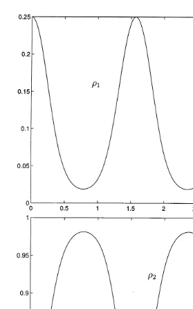
Fig. 3. Example 2.25: frequencies of the curvature tangent. The instantaneous “stationary frequencies”,!(t0) (i.e. the eigenvalues of ˆK(t0)), ofR(t; s) =12cos[cos(t)−cos(s)] +12cos[sin(t)−sin(s)]. See the following gure for the corresponding radii.
Fig. 4. Example 2.25: radii of the curvature tangent. The weights, (t0), of the tangent correlation of
R(t; s) =12cos [cos(t)−cos(s)] +12cos [sin(t)−sin(s)].
Conversely, if R is smooth, then for a xed t and any s,
xt+h−xt
h ;xs
→
h→0@tR|(t; s);
and since
xt+h−xt
h
2
=R(t+h; t+h)−2R(t+h; t) +R(t; t)
Fig. 5. Example 2.25: comparing various approximations. The upper diagram compares the coecient of the rst non-vanishing error terms in two approximations of the process X: by ˜X, the curvature tangent, and by X(has the right rst 3 curvatures). The lower diagram compares(Xt−X˜t) with(Xt−Xˆt), where ˜
Xand ˆXare the tangent, respectively, the intuitive stationary approximations at=8.
Given an s.i.d correlation or curve we dene its (innite number of ) curvatures exactly as we did in Section 2.1 for the s.n.d case. Namely, given an s.i.d correlation
R, its curvatures can be computed from (6) and (7). Alternatively, ifxis an s.i.d curve, then let {Ck(t): k= 0;1;2; : : :} be the result of the Gram–Schmidt procedure applied
to{x(tk):k= 0;1;2; : : :} (normalized so that hx (j)
t ;Cj(t)i¿0), and dene i,Vt and Kt as the innite-dimensional version of Denition 2.3. Note that the orthogonal frame,
Vt, has orthonormal rows, but is no longer necessarily an orthogonal matrix. Clearly, (3) holds, therefore the o.d.e. ˙V=KV is well dened and valid. Claim 2.5 also holds essentially unchanged. Note that, by (7) (or (5)), i is now innitely dierentiable, and that as in the s.n.d case, stationary correlations have constant curvatures.
While an s.n.d correlation can be recovered from its curvatures, this is no longer the case for an s.i.d correlation, not even in the stationary case. Therefore, in general, we cannot single out a curvature tangent, and we are led to the introduction of a slightly weaker notion.
Denition 3.2.
• A correlation, ˜R, is a curvature stationary approximation (c.s.a) to an s.i.d correlation
R, at (t0; t0), if ˜i ≡i(t0).
• A curve, ˜x, is a c.s.a to an s.i.d curve x, att0, if ˜i≡i(t0) and ˜Ci(t0) =Ci(t0).
It is important to note that, as we show in Section 3.2, an s.i.d curve x∈l2 always
has a c.s.a, ˜x, at t0 (Corollary 5), and therefore an s.i.d correlation also has a c.s.a.
The results for curves and correlations from Section 2.4 can now be trivially extended to the s.i.d case. The order of stationarity as dened in Denitions 2.19 and 2.21 remains unchanged, as do Claims 2.18 and 2.20. Replacing “stationary tangent” with “c.s.a” we obtain the s.i.d versions of Theorems 2a, 3 and 4, and Claim 2.22.
As for processes, recall that the representation (9), Xt=h;xti, allowed us to es-sentially reduce the problem of the tangent process to that of the tangent curve. The same representation holds for s.i.d processes as well. Indeed, the Karhunen–Loeve the-orem implies the existence of a vector, , of i.i.d N(0;1) random variables, and of an s.i.d curve, x, such that for each t ∈I; E[Pn
1ixi(t)−Xt]2 → 0. It follows by a result of Itˆo and Nisio (1968; Theorem 4:1), that the series Pn
1ixi(t) converges a.s.
to X uniformly on I. Moreover, since for any xed k, the same holds for the series Pn
1ixi(k)(t), as in the s.n.d case, X(k)=h;x(k)i. Thus, Denition 2.15 of the tangent process, Theorem 2b, and the process variants of Theorem 4 and Claim 2.22 all hold for s.i.d processes as well, subject to the usual proviso that “stationary tangent” should be understood as c.s.a.
3.2. Curves with constant curvatures
Remark. By considering the curve x=0 instead of x, we can assume without loss of
generality that 0≡1.
Let K be the curvature matrix of an s.i.d x. Let uk(t) be the kth column of the orthogonal frame of x, Vt. Then,
˙
Thus, the question of existence and uniqueness of a curve with a given curvature matrix K, is related to the study of the evolution equation (18). We next explore this connection in the case of a constant curvature matrix.
Let K be a curvature type matrix (Denition 2.7) and, as in the nite-dimensional case, dene ˆK by ipping the sign of the entries in the lower sub-diagonal ofK. As in the proof of Claim 2.14, letU be the unitary operator dened byUej=ijej. Then, on the subspaceL⊂l2 of nitely supported sequences,K=−U−1iKUˆ . ˆK is a symmetric
operator on L, therefore we can close it, and it is not hard to verify that its deciency indices are either (0;0) or (1;1) [Akhiezer, 1965, Section 4:1:2]. We will say ˆK (or
K) is (0;0) if these are the deciency indices of ˆK. If ˆK is (0;0) then its closure is self-adjoint and it is the unique self-adjoint extension of ˆK. Else, ˆK is (1;1) and there is a one-parameter family of self-adjoint extensions of ˆK. These self-adjoint extensions of ˆK are restrictions of its adjoint, ˆK∗, to a proper domain. It can be veried that
ˆ
K∗ is the natural operator one would associate with a matrix, i.e., ( ˆK∗u)i d
=P jKˆijuj and u ∈ D( ˆK∗) if and only if P
|( ˆK∗u)
i|2¡∞. For more on this subject see e.g. [Akhiezer and Glazman, 1981, Chapter VII].
Let ˆA be a self-adjoint extension of ˆK, and dene
A=d −U−1iAU:ˆ
Then it is easily veried that
hAej;eki=hKej;eki:
Therefore A is a skew-adjoint extension of K. Note that although K was real, with respect to the standard conjugation operator on l2, A is not necessarily so. Be that as
it may, by Stone’s theorem (e.g. [Goldstein, 1985, Chapter 1]) A is the generator of a (C0) unitary group of operators denoted by etA. That is, for any ’∈D(A), ut
d
= etA’ satises ˙u=Au andu0=’. The group etA will thus allow us to construct curves with
a given curvature matrix. One should note though, that this general theory of operators is not entirely satisfactory from our point of view, since the ode (18) is well dened, coordinate wise, even if u6∈D(A).
We are only interested in real curves, denoted by xt∈l2(R), and since, in general,
A is not real, we need:
Claim 3.3. etA’∈l2(R) for any t ∈R and ’∈l2(R) if and only if ; the spectral
measure of Aˆ with respect to e1; is symmetric; i.e.; d(x) = d(−x).
Proof. Clearly, etA’∈l2(R) for all’ and t if and only if hetAe
j;eki ∈R for all t∈R andj; k ∈N. Since
dn+m dtn+mhe
tAe
1;e1i=hetAAne1;(−1)mAme1i= (−1)mhetAKne1; Kme1i;
and since Span{e1; Ke1; : : : ; Kme1}= Span{e1; : : : ;em+1}, it follows that etA’ ∈ l2(R)
for all t and ’ if and only if hetAe
1;e1i ∈ R for all t. Let e−itAˆ be the group of
that etA=U−1e−itAˆU and therefore
for all t, which is equivalent to the symmetry of .
The next claim assures us that such symmetric spectral measures always exist.
Claim 3.4. (i) IfKˆ is essentially self-adjoint(the (0;0) case); then its spectral mea-sure with respect to e1 is symmetric.
(ii) IfKˆ is (1;1); then it has exactly two self-adjoint extensions with a symmetric spectral measure with respect to e1.
Proof. The proof is a variation on Theorem 2:13 in Simon (1998). Let W be the unitary operator dened on l2 by Wen= (−1)n+1en. ThenWKˆ∗W−1=−Kˆ∗. Let ˆA be a self-adjoint extension of ˆK, so ˆK⊂Aˆ⊂Kˆ∗. We show next thatD( ˆA) is an invariant
subspace of W, or equivalently, that
WAWˆ −1=−A;ˆ (20)
if and only if dAˆ, the spectral measure of the operator ˆA with respect to e1, is
symmetric. Indeed, if ˆA satises (20) then
dAˆ(−) = d−Aˆ() = dWAWˆ −1() = dAˆ():
Conversely, assume that d−Aˆ is symmetric and let B d
This implies that eitB= eitC for all t, and in particular their generators are identical so (20) holds.
If ˆK is (0;0), then ˆK∗ is the self-adjoint closure of ˆK whence (20) holds, and (i) follows.
Suppose, on the other hand, that ˆK is (1;1). Von Neumann theory of extensions of symmetric operators (e.g. Akhiezer and Glazman, 1981, Chapter VII) guarantees the existence of normal eigenvectors C;w ∈ l2 such that ˆK∗C= iC and ˆK∗w=−iw.
Specifying that hC;e1i¿0 and hw;e1i¿0 uniquely determines both. According to von
Neumann, any self-adjoint extension of ˆK can be uniquely characterized as follows. Choose ∈[0;2), let z=(d C−eiw)=2i, and letD( ˆA)=d D( ˆK)⊕Span{z} where⊕
stands here for a direct sum (not orthogonal). Then, ˆA, the restriction of ˆK∗ toD( ˆA) is a distinct self-adjoint extension of ˆK. Using induction, one can verify that WC=w
andWw=C. It follows that for=0 and=; D( ˆA) is an invariant subspace ofW and
which implies that D( ˆA) is not invariant under W, since by von Neumann,
D( ˆK∗) =D( ˆK)⊕Span{C} ⊕Span{w}:
This completes the proof of (ii).
LetA be a skew-adjoint extension ofK. As mentioned earlier, so far we only know that etA’ satises (18) if ’∈D(A). What if we start with ’6∈D(A)?
Claim 3.5. For any ’∈l2; u t
d
= etA’ satises d
dthut;eji=hut;−Keji for j¿1: (21)
Remark. Note that the last equation is equivalent to (18) being satised coordinate wise.
Proof. 1
h(hut+h;eji − hut;eji) =
1
hh(e
hA
−I)etA’;eji
=
ut; 1
h(e
−hA−I)e j
:
As h→0, the right-hand side converges to hut;−Aeji=hut;−Keji.
We can now prove the existence of a stationary curve with a given constant curvature matrix.
Claim 3.6. Let K be a curvature type matrix and let V0 be an orthogonal matrix.
Let A be a skew-adjoint extension of K such that dAˆ is symmetric; then the curve x= (ed tAV
0)∗e1 satises:
(i) The constant curvature matrix of x is K. (ii) The orthogonal frame ofx at t= 0 isV0.
(iii) x is a real stationary curve with correlation
R(t; s) = Z
ei(t−s)dAˆ():
Proof. Let Vt d
= etAV0 and denote its columns by uk(t); k= 1;2; : : : ; and its rows by
Cn(t); n¿0. For each k; uk(t) = etAuk(0), so by the previous claim, for j¿1
d
dthuk;eji=huk;−Keji=jhuk;ej+1i −j−1huk;ej−1i;
wheree0= 0. Therefore withd C−1= 0,d
˙
Cn=−nCn−1+n+1Cn+1:
By denition, xt = C0(t) and an elementary inductive argument shows that
Span{xt;x(1)t ; : : : ;x (n)
Since Vt is an orthogonal matrix it follows that it is the orthogonal frame of x at time
t and that K is the constant curvature matrix of x. This proves (i) and (ii). Finally, by Claim 3.3, etA is real, thus x
t∈R and
R(t; s) =hxt;xsi=hV0−1e−tAe1; V0−1e−sAe1i=he(s−t)Ae1;e1i;
which by (19) proves (iii).
The last claim shows that a skew-adjoint extension ofK can yield a stationary curve satisfying (i) and (ii) of that claim. We show next that this is the only way to get such curves.
Claim 3.7. Let x be a (real) stationary curve. Let K be the curvature matrix of x
and letVt be its orthogonal frame att.Suppose thatV0 is an orthogonal matrix,then
there exists a skew-adjoint operator A⊃K such that Aˆ is symmetric and Vt= etAV0.
Proof. As usual, let Ci(t) be the orthonormal rows of Vt. One can show by induction,
that for a stationary x (cf. Claim 2.5),
Span{x(2t k):k= 0; : : : ; n}= Span{C2k(t):k= 0; : : : ; n};
Span{x(2t k+1):k= 0; : : : ; n}= Span{C2k+1(t): k= 0; : : : ; n}:
Therefore, hx(i)(t);x(j)(s)i = (−1)i−jhx(i)(s);x(j)(t)i implies that |hCi(t);Cj(s)i| = |hCi(s);Cj(t)i|. By assumption, {Ci(0) :i¿0} is an orthonormal basis. Therefore for any i,
X
j
|hCi(0);Cj(t)i|2=X
j
|hCi(t);Cj(0)i|2= 1;
and we can conclude that Vt is an orthogonal matrix for any t. Let Uts be the linear map dened by Utsuk(t)
d
=uk(t+s), where uk(t) are the columns of Vt. Since Vt is an orthogonal matrix Uts is a well-dened orthogonal operator. Clearly Uts=Vt+sVt−1, thus
hUtsek;eji=hVt∗ek; Vt∗+seji=hCk−1(t);Cj−1(t+s)i:
Sincexis stationary,hCk−1(t);Cj−1(t+s)idepends only ons, whence for allt; Uts=U0s
which we denote byUs. It follows that Ut+s=UtUs and by Stone’s theorem Ut= etA where A is the skew-adjoint generator of the orthogonal group Ut. Since ˙V =KV, necessarily A⊃K. Finally, since Vt = etAV0 is real and V0 is orthogonal, it follows
from Claim 3.3 that Aˆ is symmetric.
Corollary 5. Let W be a row-orthonormal matrix and let K be a curvature type matrix. Then; Kˆ is either(0;0)or(1;1); according as there exist exactly one or two non-equivalent stationary curves x satisfying:
Remark. By the presumed stationarity of R, if (iii) holds at t= 0, it holds for all t. This condition is then equivalent to the fact that the Gaussian process governed by R
is completely predictable given all its derivatives at any given t.
Proof. By Claim 3.4, ˆK is either (0;0) or (1;1), according as there exist exactly one or two skew-adjoint extensionsA⊃K with a symmetricAˆ. For any suchA, by Claim 3.6,
y= (ed tA)∗e
1 is a stationary curve with a constant curvature matrix K and its orthogonal
frame at 0 is I. Let x=d W∗y. Since W∗ is an isometry, x is also a stationary curve
with the curvature matrix K, and its orthogonal frame at 0 is (W∗I)∗=W. By the denition of x, Span{xt:t ∈ R} ⊂Span{wi}, therefore x satises (i) – (iii). We next show that these are the only such curves: suppose that x is a curve that satises (i) – (iii). Then, W considered as an operator on Span{xt} is an isometry. Thus, y
d
=Wx
is a stationary curve with the curvature matrix K and its orthogonal frame at 0 is I. Therefore, by Claim 3.7,y is one of the curves considered in the rst part of the proof and so is x.
Remark. It is known that if K is (1;1), then the spectral measure, dAˆ, of any
self-adjoint extension ˆA⊃Kˆ is discrete (e.g. Simon, 1998, Theorem 5). Thus, the curves, representing the corresponding correlations are, as in the nite-dimensional stationary case, just a bunch of circular motions. This should be contrasted with the curvatures that uniquely characterize R(r) = sinr=r: there is no curve, representing R, that is composed of circular motions in orthogonal, two-dimensional, planes.
The existence of two non-equivalent stationary curves with a (1;1) constant curvature matrix K has a somewhat undesirable consequence:
Claim 3.8. If Kˆ is (1;1); then there exist non-stationary curves with the constant curvature matrixK.
Proof. Let ˆA1 and ˆA2 be the two non-equivalent extensions of ˆK with symmetric Ajˆ.
As usual, Aj=−U−1iAˆjU are the corresponding skew-adjoint extensions of K. Then, by Claim 3.6,xt
d
= (etA1)∗e 1andyt
d
= (etA2)∗e
1are two (real) stationary curves satisfying
(i) – (iii) of that claim (with V0=I). Consider the curve
zt=d
yt t60;
xt t ¿0:
Since the orthogonal frame of both x andy, at t= 0, is I, and since their curvatures are identical, it follows that z is a smooth curve with the constant curvature matrix
K. By (iii) of Claim 3.6, zis non-stationary. Note that similarly we can construct any curve z that is made of segments along whichz is alternately equivalent to x or to y.
Claim 3.9. If the curvature type matrix K is (0;0); then for any ’∈l2 there exists a unique curve u in l2 which is weakly continuous (i.e., u
t → ut0 weakly in l 2; as
t→t0); and such thatu satises(21) and u0=’.
Remark. Identifying K with its skew-adjoint closure, we know that ut= ed tK’ is a solution of (21) with u0=’. Furthermore, if we assume that ut ∈ D(K) for all t, then by the “well-posedness theorem” (e.g. [Goldstein, 1985, Section II:1:2]), u is the unique solution of the evolution equation ˙u=Ku, u0=’. Thus, it is also the unique
solution of (21).
Proof. Letu be such a coordinate wise smooth and weakly continuous solution. Dene
w(t)
as we are considering a bounded time interval where kuk is bounded by the weak continuity assumption. Therefore, as →0; w(t)→u(t) weakly in l2. Thus,
Claim 3.10. If Kˆ is (0;0); then there exists a unique correlation with the constant curvature matrixK.
uk(t) be the columns of Vt. Then, clearly, ˙uk=Kuk. Since
kuk(t)k2= X
j
hCj;eki26kekk2= 1;
and since as t→t0,
huk(t);eji=hCj−1(t);eki → hCj−1(t0);eki=huk(t0);eji;
uk is weakly continuous. Therefore by the last claim Vt= etKV0, and it follows that
R(t; s) =hxt;xsi=hV0V0∗e−tKe1;e−sKe1i=he(s−t)Ke1;e1i:
In view of the last claim, one might be tempted to guess that if ˆKt is (0;0) for all t, then there exists a unique correlation with the curvature matrices Kt. We do not know the answer to this question nor to the question whether any such curvature type matrix valued function is the curvature matrix of an s.i.d correlation. The next section mentions a dierent representation of these problems.
3.3. Curvatures and orthogonal polynomials
By now we know that the curvatures of a stationary correlation are intimately related with its derivatives, which in turn are the moments of the spectral distribution function (up to sign changes). Thus, we are naturally drawn into the classical moment problem: given a list of moments, is there a positive measure which produces them? In fact, the relation with the moment problem is more involved.
From the classical moment theory (Akhiezer, 1965), we know that a sequence{Mk} agrees with the moments of a positive measure, if and only if it is positive in the Hankel sense (i.e., P
i; kMi+kaiak¿0 for any a= (a0; : : : ; an−1)∈Rn). Such sequences are in
1:1 correspondence with innite symmetric, tridiagonal, Jacobi matrices (provided the moment sequence is normalized so that M0= 1). A convenient way to describe this
correspondence is via the orthogonal polynomials. Indeed, if a positive measure has moments of all order, then one can apply the Gram–Schmidt procedure to the powers 1; ; 2; : : : ; in the Hilbert space L2(), to get the orthonormal polynomials {P
k()} (note that the only information used in this process is the moments of the measure). In fact, one usually computes them using the famous three term recursion formula they satisfy (Akhiezer, 1965):
bkPk+1() = (−ak)Pk()−bk−1Pk−1():
The coecients in this recursion formula are the entries in the Jacobi matrix associated with the given list of moments. More precisely, the{an}n¿0 are the entries on the main
diagonal, while the strictly positive{bn}n¿0 are on the two sub-diagonals. Furthermore,
bk= p
Tk−1Tk+1
Tk
where
It is not hard to verify that symmetric positive-denite sequences (i.e., with vanishing odd moments) are in 1:1 correspondence with Jacobi matrices with vanishing main diagonal.
The similarity to the curvature computation is not a coincidence:
Claim 3.11. For stationary correlations; k=bk−1.
Proof. In the stationary case, with
R(t; s) =S(t−s) and S(r) = Z
eird();
@jt@ksR|(t; t)= (−1)kS(j+k)(0) = (−1)kij+kMj+k:
Hence, (7) can be written as,
Dk=
As in Claim 2.14, the matrices that appear in (23) and (24) are unitary equivalent, in particular Dk=Tk. Comparing (22) with (6) completes the proof.
Remark 3.12. The last claim shows the curvatures are a generalization of the Jacobi matrices to the non-stationary case, and that in the stationary case, the symmetrization of the curvature matrix, ˆK (cf. Denition 2.13), is exactly the Jacobi matrix.
The above discussion allows us to provide alternative proofs to some of the state-ments in Section 3.2. For example, Corollary 5 translates into the following statement about the classical moment problem: LetK be a Jacobi matrix with vanishing diagonal. Then there exist exactly one or two positive measures such that, is symmetric, it solves the corresponding moment problem and the polynomials are dense inL2(),
ac-cording asK is (0, 0) or (1, 1). This statement can be deduced from Akhiezer (1965), or it can be found, more explicitly, in Keich (1996, Section 5:5).
The symmetric moment problem can be equivalently stated in terms of a real positive-denite function (alternatively, a stationary correlation), as follows: given a symmet-ric sequence {Mn}, does there exist a (unique) stationary correlation R such that
R(k)(0)=(−1)kM
in terms of the deciency indices of the Jacobi matrix (cf. Corollary 5). This can be generalized as follows: given a sequence of smooth functions dened on the interval I,
{M2n(t)}, does there exist a (unique) correlationR, dened onI×I, such that for any
t∈I,@k
t@ksR|(t; t)=M2k(t)? Note that (26) below shows that{@kt@ksR|(t0; t0)}determine all
other derivatives of R at (t0; t0). As in the stationary case, an obvious necessary
con-dition for the existence of such an Ris that Di¿0, whether this is also sucient and whether there is a similar criterion for uniqueness are the same unanswered questions that were raised at the end of the previous section.
4. A few words on-curvatures
4.1. The denition
The previous sections provided us with a rather complete picture of the smooth case. This section oers a peek at our approach to the issues of non-smooth correlations as well as correlations that are given on nite time intervals. In this paper we restrict ourselves to a brief overview of the subject, a deeper study will appear in a following paper.
The basic idea is to replace derivatives with nite dierences. Let ¿0 and f be a function on R, we dene
f(t)=d f(t+=2)−f(t−=2)
:
LetRbe a continuous correlation on [−T=2; T=2]×[−T=2; T=2]. With nite dierences replacing derivatives, we dene the-curvatures ofR in a way analogous to (5) – (7). First, let
where all dierences are evaluated at 0. Hence as in the smooth case, Dk is the square of the volume of the parallelepiped generated by x0; x0; : : : ; kx0. So with D−1
d
= 1, we can dene the “-curvatures” as
provided Dk−1¿0 which is the analogue of the strong n=innite-dimensional
assump-tions. If R is n-dimensional, then, loosely speaking, for most s; Dn−1()¿0.
Remark.
• With the obvious modications, this computation can be centered about any t0.
• If R is smooth, it is not hard to see thatk() →
Remark. Note that is supported on a compact set. Thus R is indeed smooth.
The importance of -curvatures is that, in some cases, they allow us to dene
-tangents which are analogues of the tangents we dened in the nite-dimensional case.
Proof. The spectral function of R is
d(!) = 1
d!
1 +!2:
By Claim 4.1, it suces to show that the curvatures of =◦S−1 are as advertised. As explained in Claim 3.11, this is equivalent to nding the Jacobi matrix associated with . The latter is computed in Keich (1999, Example 6:1).
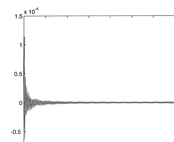
Using a dierent technique, we can prove that the-curvatures, att0, of the Brownian
Fig. 6. Distance between 2e−|r|=4 and the-tangent tot∧s. The intuitively expected tangent to the Brownian motion correlationt∧s, att0= 2, is the correlation ˜R(r) = 2e−|r|=4. The gure depicts the relative distance between ˜Rand the-tangent, whereT= 1; n= 321 and=T=(n−1). Other choices oft0yielded essentially the same picture.
The proof of this claim will appear in the aforementioned paper dedicated to the study of the discrete case. It turns out thatnumerically, the-tangents of the Brownian motion correlation about the pointt0 converge, as→0, to an Ornstein–Uhlenbeck correlation:
˜
R(r) =t0e−|r|=2t0. Fig. 6 provides a typical example of the quality of approximation that
was observed. Note that this result agrees with our intuition, since if you normalize R
to have a constant variance, you obtain a time changed Ornstein–Uhlenbeck correlation:
R(t; s)
√
t√s = e
−12|log(t)−log(s)|;
and for t; s near a xed t0 (cf. Example 2.23),
e−12|log(t)−log(s)|∼e−|t−s|=2t0:
5. Somewhat technical claims and their proofs
Claim 5.1. Let R be an s.n.d correlation and let
Let {pk}mk=0⊂N be a strictly decreasing sequence. Then there is a perfect equiva-the last inequality is due to equiva-the monotonicity of{pi}. This proves one half; the other implication is proved by induction on m.
For the base of the induction letm= 0. Here N0=20, and Hence this term has been determined by the corresponding {Nk(p)}. As for the second term, can determinen(t) = 0 fromNn (as the previous curvatures are all positive). Once we determine n≡0, the subsequent curvatures have to be 0 by denition.
Proof of Claim 2.20. By Claim 5.1, it suces to show that {@kR|(t0; t0):k6n} are in
perfect equivalence with {Nk(p)(t0): 06k6[n=2]; 06p6n−2k}. In order to do so, it
is convenient to change coordinates: let = (t−s)=2 and= (t+s)=2. As an example of the equivalence we seek to prove, consider the case n= 2: one can verify that,
R(t; t) =N0(t);
This equality holds for any smooth R, and by the same token
@p@2mR|(t; t)=
References
Akhiezer, N.I., 1965. The Classical Moment Problem and some Related Questions in Analysis. Hafner Publishing Company, New York.
Akhiezer, N.I., Glazman, I.M., 1981. Theory of Linear Operators in Hilbert Space. Pitman, London. Goldstein, J.I., 1985. Semigroups of Linear Operators and Applications. Oxford University Press, Oxford. Itˆo, K., Nisio, M., 1968. On the convergence of sums of independent Banach space valued random variables.
Osaka J. Math. 5, 35–48.
Keich, U., 1999. Krein’s strings, the symmetric moment problem, and extending a real positive denite function. Comm. Pure Appl. Math. 52 (10), 1315–1334.
Keich, U., 1996. Stationary approximation to non-stationary stochastic processes. Doctoral dissertation. Courant Institute of Mathematical Sciences.
Krein, M.G., 1940. On the continuation problem for Hermitian-positive continuous functions. Dokl. Akad. Nauk SSSR 26, 17–21.
Krein, M.G., 1944. On the problem of continuation of helical arcs in Hilbert space. Dokl. Akad. Nauk SSSR 45, 147–150.
Loeve, M., 1963. Probability Theory, 3rd Edition. Van Nostrand, Princeton, NJ.
Mallat, S., Papanicolaou, G.C., Zhang, Z., 1998. Adaptive covariance estimation of locally stationary processes. Ann. Statist. 26 (1), 1–47.
von Neumann, J., Schoenberg, I.J., 1941. Fourier integrals and metric geometry. Trans. Amer. Math. Soc. 50, 226–251.
Priestley, M.B., 1988. Non-linear and Non-stationary Time Series Analysis. Academic Press, New York. Priestley, M.B., 1996. Wavelets and time-dependent spectral analysis. J. Time Ser. Anal. 17 (1), 85–103. Simon, B., 1998. The classical moment problem as a self-adjoint nite dierence operator. Adv. in Math.
137 (1), 82–203.