Received March 21, 2016 Published as Economics Discussion Paper June 23, 2016
Vol. 10, 2016-31 | November 28, 2016 | http://dx.doi.org/10.5018/economics-ejournal.ja.2016-31
Prudential Regulation in an Artificial Banking
System
Pedro Dias Quinaz and José Dias Curto
Abstract
This study is an exploratory analysis of the economic role of banks under different prudential frameworks. It considers an agent-based computational model populated by consumers, firms, banks, and a central bank whose out-of-equilibrium interactions replicate the conjunct dynamics of a banking system, a financial market and the real economy. A calibrated version of the model is shown to provide an intelligible account of several recurring economic phenomena, thus constituting a favorable ground for policy analysis. The investigation provides a valuable methodological contribution to the field of banking research and sheds new light on the role of banks and their prudential regulation. Specifically, the results suggest that banks are key economic agents. Through their financial intermediation activity, credit institutions facilitate investment and promote growth.
JEL C63 G28
Keywords Agent-based computational model; financial intermediation; prudential policy; bank regulation
Authors
Pedro Dias Quinaz, University of Lisbon, Lisbon, Portugal
José Dias Curto, University of Lisbon, Lisbon, Portugal, [email protected]
Citation Pedro Dias Quinaz and José Dias Curto (2016). Prudential Regulation in an Artificial Banking System.
Economics: The Open-Access, Open-Assessment E-Journal, 10 (2016-31): 1—54. http://dx.doi.org/10.5018/
1
Introduction
Are banks key drivers of economic performance? What are the effects of different macro and micro-prudential regulations on economic growth? These seminal questions have resurfaced in the aftermath of the 2008 financial debacle as a central topic in banking research and as an important source of concern for policy makers. In this study we develop an agent-based computational model through which an exploratory analysis of the economic role of banks under different prudential frameworks is conducted.
The years that preceded the 2008 crisis were characterized by blatantly reckless mortgage lending. Loan-underwriting criteria were so lenient that “subprime” borrowers with no capacity to redeem their debt had easy access to credit. These mortgages were pooled together and used to back collateralized debt obligations (CDOs). As soon as the housing markets collapsed, “domino effects” spread throughout the extremely interconnected financial system, quickly exposing severe fragilities. The price of mortgage-backed securities fell dramatically, and allegedly safe CDOs were, in the end, worthless. The sale of such securities or their use as collateral became increasingly difficult. In an effort to rally liquidity, banks started to sell assets at fire-sale prices, giving rise to “price spiral” phenomena that, in turn, reduced banks’ capital thanks to “mark-to-market” accounting rules. When banks started doubting the solvency of their counterparties, wholesale agents stopped rolling over short-term debt, causing the failure of banks that had relied on non-stable sources of funding (The Economist, 2013).
The financial system proved to be incredibly fragile. Banks had expanded more than ever before, leveraging beyond reasonable levels and holding insufficient capital to absorb losses. It is, therefore, no surprise to note that the ex-post analysis of the failed mechanisms that led to the crisis has focused on banks’
raison d’être and on the regulatory instruments that can increase and promote
financial stability.
information between investors and firms. Banks also provide maturity transformation, a process whereby short-term liabilities are converted into long-term assets (Freixas and Rochet, 2008). The literature postulates that agency problems (Dewatripont and Tirole, 1994) and the risk of a systemic crisis (Santos, 2001) are the main reasons why banks should be subject to regulatory requirements.
Across time, several were the instruments - one of the most prominent ones being the deposit insurance scheme proposed by Diamond and Dybvig (1986) – suggested by academia to mitigate or prevent the negative effects of bank bankruptcies. In spite of this, and due to its function in reducing risk-taking and providing a buffer to absorb losses, the regulatory spotlight always fell more brightly upon bank capital (Allen and Gale, 2007). In this regard Basel III/CRD IV rules, which are at present mandatory for Euro area banks, represent the latest regulatory effort to ensure the robustness of the banking system. Besides the enhancement of minimum capital requirements to at least 10.5% of risk-weighted assets, it is worth highlighting Basel III’s introduction of a counter-cyclical capital buffer. However, the latest Basel Accord is not completely consensual. Carmassi and Micossi (2012), for instance, argue that Basel III could follow a much simpler path in route to a more stable financial system simply by abandoning the risk weighting approach.
The strong debate surrounding prudential policies, coupled with the blatant failure of macroeconomic models in the 2008 financial crisis, suggests that the study of regulatory policies is not within the grasp of the existing nucleus of mainstream economic knowledge. The notions of interdependence, networks, trust and expectations, which are key to understanding the financial crisis, appear not to be “features of modern macroeconomic models” (Kirman, 2010: 501). To address these shortcomings, it is crucial that economists start considering the economy as a complex evolving system (Taylor, 2007). This can be done through agent-based modeling, a technique that allows researchers to simulate and comprehend out-of-equilibrium economic dynamics (Arthur, 2006).
can exhibit emergent phenomena that cannot be foreseen or understood by any agent on an individual level. Instead of modeling economies under the omniscience assumption, according to which the decisions of agents are pre-coordinated, agents are programmed to follow simple behavioral rules that may or may not result in equilibrium. Through computer simulations the behavioral patterns of the system can be scrutinized and understood. Once a computer program able to replicate the phenomena of interest is developed, researchers can use it as a laboratory in which they can conduct policy experiments.
In this vein, it is the purpose of this paper to assess, through the use of a rich, yet tractable agent-based model, the effectiveness and efficiency of prudential regulatory measures in their effort to maintain a stable and sound banking system. We add to the literature by creating a stylized agent-based computational model1 that simultaneously replicates the conjunct dynamics of a financial market, a banking system and the real economy, mimicking several stylized facts of the latter and grasping, to a certain extent, the implications of banking regulation in economic performance.
The conceptual framework employed draws heavily from Takahashi and Okada (2003) and Tedeschi et al. (2012). For tractability, we adopt a parsimonious approach that drifts away from fully specified models such as the Eurace project (Raberto et al., 2012; Cincotti, 2012). Specifically, our model attempts to depict, in an admittedly stylized form, the inner workings of a small economy comprising consumers, firms, commercial banks and a central bank. Consumers are responsible for providing the work force needed for production and for driving internal demand through consumption. Firms are profit-maximizing entities that produce the consumption good and are thus responsible for driving supply. The primary function of banks is to collect deposits from their clients and to give out loans to consumers and companies. Banks are also subject to prudential rules and regulations established by the Central Bank (i.e., minimum capital ratios and minimum loan underwriting standards).
Following Ashraf et al. (2011), the model is calibrated to U.S. data. Simulations are repeatedly performed, for several time periods and under diverse
_________________________
1 The agent-based computational model has been developed in NetLogo, a multi-agent
parameter settings to assess how credit institutions affect macroeconomic performance and how performance, in turn, is affected by diverse regulatory frameworks.
With this model model we seek to make a valuable methodological contribution to the field of banking research, shedding new light on the role of banks and bank regulations by leveraging on the advantages of agent-based computational modeling. In spite of being too simple to suit the policy-making endeavor, it does generate five results of broad-spectrum qualitative interest.
The first result corroborates the view that credit institutions are crucial economic agents in so far as their existence greatly improves the performance of the economy. Banks foster growth by providing credit and expanding firms’ investment opportunities, which are usually limited to each company’s ability to endogenously generate cash flows. The capacity of the economy supply-side to meet aggregate demand is thus substantially improved when a banking system is in place. The role of credit institutions is also relevant in mitigating the negative externalities of firm failures. By providing financing to new entrants and sustaining incumbent firms by preventing capital erosion, banks are often able to alleviate the effects of shocks.
Our second result reveals that the macroeconomic impact of credit institutions and bank regulation often contradicts the traditional dogmas behind micro-prudential policies. In particular, the experiments conducted show that aggregate macroeconomic performance deteriorates as banks become safer (i.e., as stricter capital requirements are imposed). This is because decreased credit availability hampers the creation of value by reducing the speed at which supply can meet surges in demand. Furthermore, increased leverage does not always entail augmented firm bankruptcies. If credit levels are not excessive, bank funding can prevent the depletion of firms’ production capacity in periods of low demand, thus contributing to a reduction of bankruptcies in the long run. Finally, increased capital requirements do not always mean that banks are less likely to fail. Indeed, micro-prudential policy is shown to entail calibration risk: while raising capital requirements increases the immediate loss-absorbency capacity of banks, it also decreases their ability to endogenously generate capital through profits.
output gap is closed more quickly if banks are allowed to require lower financial autonomy ratios from customers and are subject to lower capital adequacy ratios. In other words, credit is proved to be more important when the output gap is greater.
A corollary of this result is that using the credit-to-GDP ratio as a trigger for the implementation of the counter-cyclical capital buffer might be an insufficient approach if taken alone. Since the same level of leverage may be too high or too low depending on the current state of the economy (i.e., the magnitude of the output gap), the establishment of a counter-cyclical capital buffer must also consider the impact of credit-constraining measures in GDP growth and an assessment of the level of debt that can be sustained by the economy without causing the build-up of system-wide risk.
More importantly, our fourth result argues, under the premises of our model, that the counter-cyclical capital buffer should never actually be implemented. Indeed, our experiments fail to find evidence in support of the rationale behind macro-prudential tools. This conclusion is not surprising if considered together with previous insights, which showed that riskier banks promote growth in fundamentally all scenarios.
Finally, our fifth result suggests that effective resolution is crucial. Specifically, resolution of credit institutions acts to the benefit of the economy by ensuring that depositors are never bailed-in to a great extent and by getting rid of “zombie-banks” that are not able to support investment.
2
A stylized model of the banking system
2.1
Conceptual framework
The conceptual framework employed draws heavily upon Takahashi and Okada (2003) and Tedeschi et al. (2012). The model depicts, in an admittedly stylized form, the inner workings of a small economy composed of I consumers, E companies (also referred to as firms), B commercial banks, and a central bank. Consumers are indexed by i = 1, … , I, companies are indexed by e = 1, … , E and banks are indexed by b = 1, …, B. Since there is no government, there are also no taxes or public expenditure.
In this economy there is only one kind of product valued by the population – the consumption good. Consumer goods are perishable and have their priced fixed at unity.
Two types of production factors exist: labor and capital. Consumers provide labor and receive compensation from companies in return. Based on their disposable income, net worth and bank deposits, consumers determine how much to spend on the consumer good. Companies decide how much to produce based on their production capacity and expectations of demand. During this process firms can invest in infrastructures and technology, increasing their productivity. In general, supply and demand (both internal and external) for the consumer good do not balance, giving rise to demand rationing (excess demand) or production waste. Economic agents can also invest in financial assets (i.e., bonds), with each debt security generating interest income at each time step. This asset is finite and exogenous to the economy, and can therefore be interpreted as a debt security issued by a sovereign country. Each consumer and company can buy and sell the financial asset in the market.
Bank deposits must mediate all transactions, and proprietors are not able to lend or borrow among themselves. Each bank grants credit and accepts deposits from their customers, with depositors being allocated randomly across banks so that each credit institution starts off with the same number of clients. Transaction settlements are executed by changing the holder of the bank deposit.
2.1.1 Consumers
Consumers are responsible for providing the work force needed for production – for which they receive their wage (�) – and for driving internal demand through consumption. They are members of the cooperative firms in which they are employed and are thus entitled to a share of their profits. In addition, consumers are also a large part of the financial asset market since they are able to buy and sell debt securities.
At each time step �, the assets of consumer � are composed of ���� units of the debt security and a bank deposit (����,�). Since companies may not always be able to fulfill their commitments to their employees, circumstances might arise in which the consumer is also owed a part of its salary (����,�). To finance the acquisition of the asset, consumers can make use of bank loans (����,�).
The value of the financial asset is marked to market at each time step:
����� =������ (1)
Hence, the net worth (i.e., the net equity) of each consumer equals:
���� =�����+����,�+����− ����,� (2)
The financial autonomy ratio of consumer � can thus be represented as:
���� = ��� �
�����+��
��,�+����
(3)
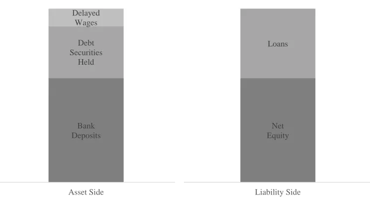
Finally, at each time step �, each consumer has a balance-sheet similar to the one depicted in Figure 1.
2.1.2 Companies (also referred to as firms)
Companies are profit-maximizing entities of a cooperative nature (i.e., owned by their employees) that produce the consumption good and are thus responsible for driving supply. The production activity entails the use of two production factors: labor and capital. While the amount of labor is fixed (i.e., each firm has�
Figure 1: Consumer’s stylized balance sheet
in order to increase its production capacity. Companies are also assumed to be able to invest in the financial asset.
At each time step �, company � owns ���� units of the financial asset, a bank deposit (����,�) and ��� of productive capital. In order to finance the acquisition of the asset or increase the production capacity through investment, companies can make use of bank loans (����,�). Finally, and since companies may not always be able to fully remunerate employees for their work, circumstances might arise in
which delayed wages are accumulated (∑ ����,�
� �
�=1 , where ����,� represents the amount of delayed wages between company � and consumer �).
Taking into account that the value of the financial asset is marked to market at each time step, the net equity of each firm equals, at time step t:
����=������+����,�+���− ����,�− � ����,� �
�
�=1
(4)
The financial autonomy ratio of company e can be represented as: Bank
Deposits Debt Securities
Held Delayed
Wages
Asset Side
Net Equity
Loans
��
��=
��
� ��
���
��+
�
��+
��
��,�(5)
Finally, at each time step t, each company has a balance-sheet similar to the one depicted in Figure 2.
Figure 2: Company’s stylized balance sheet
2.1.3 Banks
The primary function of banks is to collect deposits from their clients and give out loans to consumers and companies. This financial intermediation activity is undertaken by charging interest on loans and remunerating deposits at a lower rate. Loans are made with full recourse and are collateralized by all the assets of the borrower.
While conducting its operations the bank is subject to mandatory capital requirements and, just like an individual consumer, settles all its transactions through the exchange of deposits.
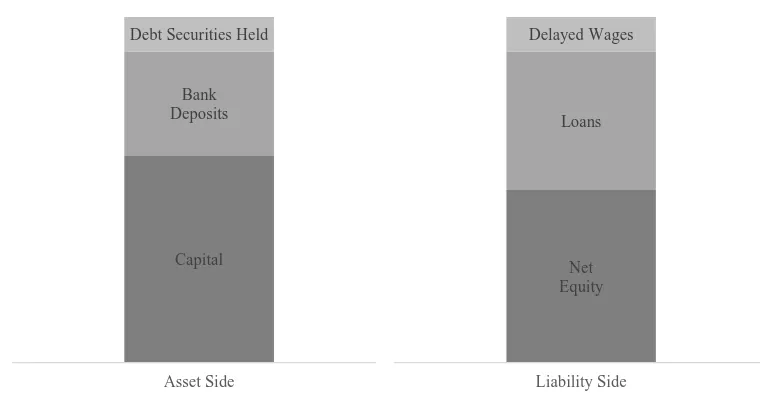
Capital Bank Deposits Debt Securities Held
Asset Side
Net Equity
Loans Delayed Wages
At each time step �, bank �’s assets comprise ���� units of the financial asset,
other hand, the liability side comprises the shareholders’ equity and retail deposits
(∑ ����,�
Taking into account that the value of the financial asset is marked to market at each time step, the net equity of each bank equals:
��� =������+����+� ����,�
The capital adequacy ratio of bank � can be represented as:
���� = �� �
�����
(7)
where the risk-weighted assets (�����) represent a risk-based measure of the bank’s exposures obtained by multiplying the value of the credit institution’s assets by a risk-weight (��) that varies according to the level of each investment’s perceived risk.
The balance-sheet of a bank is depicted in Figure 3.
_________________________
Figure 3: Bank’s stylized balance sheet
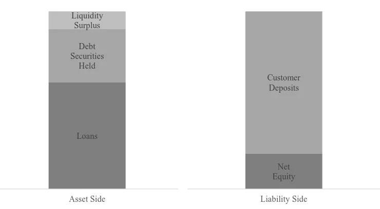
2.1.4 Central bank
In the model’s economy the central bank is primarily responsible for banking regulation and supervision. The central bank thus regulates banks and is responsible for ensuring their compliance with prudential requirements.
Specifically, the central bank requires each bank to: (i) implement specific loan underwriting policies (as defined by the minimum financial autonomy ratio demanded from customers) and (ii) maintain capital at least equal to a percentage of the value of its risk-weighted assets (bank loans and financial assets). The minimum capital adequacy ratio is represented by ������ . Credit institutions that do not comply with this prudential requirement are declared to be in financial distress and are prohibited from granting any new loans. In addition, banks with negative equity are forced into failure by the regulator, giving rise to potential losses for depositors and to the entrance of a new player.
Loans Debt Securities
Held Liquidity
Surplus
Asset Side
Net Equity Customer
Deposits
2.2
Protocol and behavioral rules
As usual in the ABM literature, and for the purpose of reducing its computational burden, the model follows a choreographed protocol that restricts the decisions taken by agents and forces them to initiate actions through 11 sequential stages:
1. Determination of internal demand for the consumption good; 2. Determination of external demand for the consumption good; 3. Determination of supply for the consumption good;
4. Loan underwriting;
5. Assessment of companies’ financial position; 6. Companies’ bankruptcy and entrance; 7. Assessment of consumers’ financial position; 8. Assessment of banks’ financial position; 9. Banks’ bankruptcy and entrance; 10. Purchase and sale of the financial asset;
11.
Distribution of profits.
Each of these steps is described in detail below.
1. Determination of internal demand for the consumption good
The level of consumption is assumed to be determined as a function of the consumer’s disposable income and net worth at the beginning of the period:
��� =��� �����−1� +����−1� �× (1 +�);���−1�,� �
�~�(0,�)
(8)
where � represents the marginal propensity to consume from income, � represents the marginal propensity to consume out of net wealth, and � is a normally distributed random variable that accounts for all other motives that may increase or decrease consumption. It should be noted that consumption is always limited by the amount of cash (i.e., bank deposits) the consumer owns at the beginning of the period.
2. Determination of external demand for the consumption good
���=��−1� × (1 +�0+ �)
�~�(0,�) (9)
where θ is a normally distributed random variable that accounts for the myriad of factors that may affect exports at each moment in time.
3. Determination of supply for the consumption good
Companies plan their production activity based on the observed last period’s demand. Demand is assumed by firms to increase at a constant rate, thus mimicking long term expectations of economic growth. Since producers are undifferentiated, expected internal demand is equally distributed across firms:
�[�]��=�∑��=1��−1�
� +��−1� �× (1 +�0) (10)
To produce the consumer good, companies use capital as the only input. Each firm can produce according to the following production function:
���=���� (11)
For simplicity purposes, capital productivity � is assumed to be constant and uniform across companies. In addition, capital is assumed to depreciate at a constant rate (�) at each time step.
Companies will initially try to produce as much as their expected demand. Since the only external source of finance that firms have are bank loans, firms will apply for credit whenever their capital is not enough to meet expected demand.
However, since borrowing entails the risk of default, each company takes into account its probability of failure when submitting a loan application.3 Credit demanded by company � to bank � is thus established according to:
_________________________
���∗,�=�� �1− expected profits and ������������+1 represents the firm’s expected debt servicing costs.
4. Loan underwriting
Credit granting is determined as a function of the financial situation of the borrower and the capital position of the bank. In an effort to replicate the “restricted lending” problems typical of the recent financial crisis, credit institutions with adequate capital are assumed to be more willing to take risks, whereas banks with inadequate capital become reluctant to lend funds. The level of loan affordability depends on the capital ratio of the bank and takes on the value zero if its capital ratio (����) stays below ������ or the capital ratio of the borrower (���) is below �����. Naturally, the bank must also have liquidity surpluses (i.e., cash holdings) to underwrite the loan. The amount of credit to be granted by the bank4 is thus defined as follows:
����=
Interest rates are assumed to be determined exogenously as a result of competition, changing as a result of the excess demand or supply of funds in the financial market. In particular, the interest rate on deposits negatively depends on the amount of deposits held by banks:
_________________________
the loan application amount is reduced. This “financial fragility” aspect is reflected in the first term of Equation (12).
��= 2 ×�̅
where �̅ represents the average interest rate on deposits and �̅ the average level of consumption.
Since loans to domestic investors involve the risk of bankruptcy, banks charge higher interest rates on loans. The rate is bank-idiosyncratic and inversely correlated to the financial robustness of the institution:
���,� =��+�×
where � is a representative parameter of the bank’s risk aversion.
All loans are based on variable interest rates, which means that the interest rate charged on the outstanding balance varies as market interest rates change. In addition, all loans are initially given out with a standard maturity �. When a consumer or a company increases the amount of borrowings received from the bank, the total amount of debt commitments is, in a process akin to debt restructurings, merged into a single loan that will mature within � timesteps.
Loans are considered to be in distress when at least one payment has been missed. Each bank determines a liquidation rule such that each of their customers goes bankrupt whenever they miss ���� consecutive payments.
5. Assessment of companies’ financial position
After trying to sell their production in the market, companies assess their cash in-flows and start making their payments. At this point, each firm’s revenues5 are given by the remuneration generated by each unit of bonds owned and the minimum between real demand and the company’s production:
_________________________
���ℎ��������= min�∑ ��−1
On the other hand, cash outflows6 are given by:
���ℎ���������=��+� �×��+��,�×����,�+���
� represents the loan’s principal repayment.
Whenever cash outflows are greater than cash inflows plus the company’s deposits, the firm gives priority to the payment of wages. Bank loans are assumed to be paid last. Amounts not paid are registered as liabilities and need to be paid in the following time step. In an effort to re-balance its financial position, the company will also try to sell any bond it owns.
Finally, the company net worth is updated as follows:
����=���−1� +���ℎ��������− ���ℎ��������� (18)
6. Companies’ bankruptcy and entrance
As already stated, banks will liquidate debtors as soon as they miss ���� payments. In such situations, the remaining company’s assets are seized by the bank and the player leaves the market.
The model assumes a simple entry mechanism based on one-to-one replacement. As such, firms that go bankrupt are automatically replaced by new players. From the empirical literature (Bartelsman and Scarpetta, 2005), new entrants are usually smaller than existing firms. Specifically, the stock of capital of
_________________________
new firms is drawn from a uniform distribution with �= min(��1,��2, … ,���) and
�= median (��1,��2, … ,���).
7. Assessment of consumers’ financial position
At this stage, the income of consumer � in period � (���)7 is a function of its wage
and the amount of bonds it owns. This can be represented as:
��� =�+������ ���� (19)
Note that the consumer might not always receive the totality of its wage, as the company for which it works might be in financial distress.
On the other hand, the cash outflow8 of each consumer at time step � is given
by:
���ℎ���������=���+��,�×����,� (20) where ��� represents consumption and ��,�×���,� represents funding costs.
Whenever cash outflows are greater than income plus the consumer’s deposits, the consumer gives priority to the liquidation of consumption expenses. Bank loans are assumed to be paid last. Amounts not paid are registered as liabilities and need to be paid in the following time step. In an effort to re-balance its financial position, the consumer will also try to sell any bond it owns.
Finally, the consumer’s net worth is updated as follows:
���� =���−1� +���− ���ℎ��������� (21)
_________________________
7 Consumer’s income also includes interest received on deposits and potential cash-inflows stemming from the sale of debt securities and from firm dividends. At this point, however, it is not possible to know whether the revenue generating capacity of the consumer’s bank is enough to meet the totality of its commitments. Interest revenue is thus added to the consumer’s net worth after the computation of the bank’s financial position (refer to Stage 8). In addition, proceeds from the sale of debt securities are added to the consumer’s bank deposits whenever a transaction is settled (refer to Stage 10). Cash inflows associated with firm dividends are added to the consumer’s net worth at the end of each time step (refer to Stage 11).
8. Assessment of banks’ financial position
At each time step banks will assess their cash-flows to determine the robustness of their financial position. Cash inflows9 consist fundamentally of interest income
and are thus a function of the debtors’ ability to service their debt and the rate of remuneration of the bank’s claims on other (foreign) credit institutions:
���ℎ�������� =����,�×����,��
In accordance with commercial banks’ business models, cash outflows10 consist of interest expenses related to the remuneration of deposits:
���ℎ��������� =����×����,��
Liquidating distressed borrowers is needed for banks to raise liquidity, thus playing a crucial role in banks’ financial stability. As already stated, banks will liquidate debtors (consumers or companies) as soon as they miss ���� payments. In this process credit institutions take over any bond still owned by the debtor11
and immediately try to sell it on the market. The transfer of the collateral’s ownership implies a direct write off of the bad loan.
Whenever cash inflows are greater than cash outflows plus the bank’s cash holdings, it is clear that the credit institution is able to meet the totality of its commitments. The net worth of both companies and consumers is thus increased by their respective remuneration on deposits:
���� =����+������,� (24)
_________________________
9 Banks’ cash-inflows also include potential revenues stemming from the sale of debt securities. Such proceeds are added to the banks’ deposits whenever a transaction is settled (refer to 10). 10 Banks’ cash-outflows also include potential payments stemming from the purchase stage of debt securities. Such disbursements are deducted from the banks’ bank deposits whenever a transaction is settled (refer to 10).
���� =����+������,� (25) Finally, the bank net worth is updated as follows:
����=���−1� +���ℎ��������− ���ℎ���������− �����+��×����� (26)
where ����� stands for the non-performing loans that were written off by bank � in time step � and ����� represents the number of debt securities foreclosed during the same time step.
9. Banks’ bankruptcy and entrance
Bankruptcy is assumed to happen to banks whenever credit institutions are not able to fulfill the totality of their commitments (i.e., whenever cash outflows are greater than cash inflows plus the bank’s cash holdings) or whenever their capital ratio is below zero. The model thus captures the possibility for both liquidity and solvency related default events.
In the event of bankruptcy, the credit institution enters into resolution. As part of this process, non-performing loans (i.e., loans with ����� > 0) are foreclosed. Debtors that were not able to fully pay their obligations to the bank see their holdings confiscated. Since the collateral’s value may not be enough to fully compensate non-performing loans outstanding, the bank’s capital might be further reduced during this process.
After all the non-performing loans are foreclosed, the capital position of the bank is assessed. Losses are first absorbed by equity capital. Depositors are bailed-in whenever equity capital is negative. Sbailed-ince all depositors have the same level of seniority, losses are distributed among all clients proportionally to the amount of deposits they own.
10. Purchase and sale of the financial asset
Supply and demand for the financial asset are generally determined by how attractive the bond is vis-à-vis other financial assets (loans). For each agent, the attractiveness of the debt security in period �, denoted by ��, is given by:
�� =��+ (2�1�� − �)− ��� (27) where
�� =
���� ×��+ �2��(��−��− ��−1)
��−1
(28)
and
��~�������� 0 ��� 1 (29) The first term on the right-hand side of Equation (28) represents the expected income accrued from owning one unit of the financial asset. The second term captures the expected capital gain perceived by the trend chasers augmented by �2, the strength of the trend-chasing attribute. Expected capital gains in Equation (28) reflect the change in the asset price over the last � − �� periods. Even though all traders are trend chasers, the capital gain term is weighted by a random variable (��) to capture divergent expectations.
The gains from holding debt securities (first term of Equation (27)), minus loan interest (denoted by the third term), measure the marginal net gain from owning an additional bond. In reality, other factors affect purchase and sale decisions: the second term of Equation (27) represents such factors. This second term further helps traders to form different expectations.
The owner attempts to sell one bond when it judges bonds to be less attractive (i.e., less than �̅), or when it is pressed to sell due to a financial distress situation. For ��� ≥1, supply of bonds (����) is such that:
���� =�10 ���� <�̅⋁��ℎ���������� > 0 ⋁��� < 0 (30)
����=�10 ��ℎ���������� >�̅ (31)
After defining its interest in buying the financial asset, every agent needs to determine if it needs bank financing. Buy-side players’ intention to acquire debt securities is limited to the purchase of one unit.
After each agent determines its market positioning, supply and demand meet randomly, resulting in transactions. The short side of supply or demand determines the actual quantity of units traded. Agents that manage to settle their transactions see their financial position updated accordingly:
��� =���− ��×���+��×��� (32)
where ��� represents the amount of debt securities purchased and ��� represents the amount of debt securities sold.
In general, prices are assumed to be sticky. The price, therefore, responds to the difference between supply and demand (��), with � representing the speed of the price adjustment:
�� =���+��−1 (33)
where
��=��−1×max(∑ ���∑ ����− ∑ ����
�,∑ ����) (34)
11. Distribution of profits
At the end of each time step, in accordance with their cooperative nature, firms distribute dividends. The payout ratio is a function of both the firm’s current cash holdings and the outflows that the company expects to face in the next period. Specifically, expected disbursements reflect each firm’s forecasted personnel and investment costs. Mathematically:
����������= max�����,�− ���×� − ��+� �×�� −�
[�]�+1� − ��+1�
� �, 0� (35)
investment opportunities or, in other words, the target capital structure of greenfield projects).
Naturally, and in case the distribution of profits is compatible with the liquidity position of each company, the net worth of each of its associates must be updated with their respective share of the dividend:
����=����+ ��������� �
� �+�
(36)
Finally, each company’s net worth is updated as follows:
����=����− ���������� (37)
2.3
Model calibration
As demonstrated above, the model has multiple individual agents. In order to restrain the number of parameters and to facilitate calibration, ex-ante symmetry between agents was imposed. In spite of the homogenous initial setting, the economy develops heterogeneous behaviors and results due to the impact of feedback effects and noise.
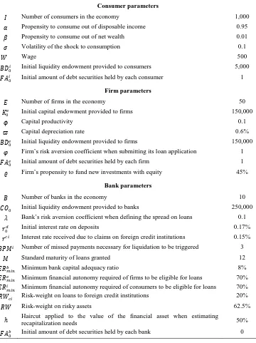
The calibration procedure follows the methodology described in Ashraf et al. (2011) and assumes that each time step represents one month. The 39 parameters of the model were classified as consumer parameters, firm parameters, bank parameters, financial market parameters, and general parameters. These are listed in Table 1 along with the assigned values under the baseline scenario. A comprehensive list of the model’s variables is also provided in Table 2.
Table 1: Calibrated model parameters
Consumer parameters
� Number of consumers in the economy 1,000
� Propensity to consume out of disposable income 0.95
� Propensity to consume out of net wealth 0.01
� Volatility of the shock to consumption 0.1
� Wage 500
��0� Initial liquidity endowment provided to consumers 5,000
��0� Initial amount of debt securities held by each consumer 1
Firm parameters
� Number of firms in the economy 50
�0� Initial capital endowment provided to firms 150,000
� Capital productivity 0.1
� Capital depreciation rate 0.6%
��0� Initial liquidity endowment provided to firms 150,000
� Firm’s risk aversion coefficient when submitting its loan application 1
��0� Initial amount of debt securities held by each firm 1
� Firm’s propensity to fund new investments with equity 45% Bank parameters
� Number of banks in the economy 10
��0 Initial liquidity endowment provided to banks 250,000
� Bank’s risk aversion coefficient when defining the spread on loans 0.1
�0� Initial interest rate on deposits 0.17%
��� Interest rate received due to claims on foreign credit institutions 0.15%
���� Number of missed payments necessary for liquidation to be triggered 3
� Standard maturity of loans granted 12
������ Minimum bank capital adequacy ratio 8%
������ Minimum financial autonomy required of firms to be eligible for loans 70%
������ Minimum financial autonomy required of consumers to be eligible for loans 70%
���� Risk-weight on loans to foreign credit institutions 20%
�� Risk-weight on risky assets 62.5%
ℎ Haircut applied to the value of the financial asset when estimating recapitalization needs 50%
Financial market parameters
�� Coupon rate of the debt security 0.17%
���� Notional amount of the debt security 300,000
�0 Initial price of the financial asset 2055
� Agents’ propensity to form divergent expectations regarding the financial asset price 0.5
�1
Agents’ propensity to form divergent expectations regarding the financial
asset price 0.2
�2 Strength of the trend-chasing attribute 1
�̅ Attractiveness threshold for the financial asset 0.01
� Price adjustment speed 0.1
General parameters
�0 Expected growth of internal and external demand 0.26%
�0 Initial amount of external demand 56,000
Table 2: Model variables
Consumer variables
����,� Wages in arrears
���� Debt securities held
����,� Outstanding bank loans
����,� Bank deposits owned
����� Mark-to-market value of the financial assets held
���� Consumer’s net worth
���� Financial autonomy ratio
��� Level of consumption
��� Disposable income
�̅ Average level of consumption
Firm variables
���� Debt securities held
����,� Bank deposits owned
��� Productive capital
���� Firm’s net worth
���� Financial autonomy ratio
��� External demand
�[�]�� Expected internal demand
��� Firm’s production
����+1
�������� Expected debt servicing costs
�[��+1] Expected profits
Bank variables
���� Debt securities held
���� Cash holdings
��� Net equity
���� Financial autonomy ratio
����� Risk-weighted assets
���∗ Loan amount required by the applicant
�� Interest rate on deposits
�̅ Average interest rate on deposits
���,� Interest rate on loans
����� Foreclosed financial assets
����� Written-off non-performing loans
Financial market variables
�� Price of the financial asset
���� Supply for the financial asset
���� Demand for the financial asset
��� Bonds purchased
��� Bonds sold
�� Difference between supply and demand
2.3.1 First stage of the calibration
Consumer parameters. Following Takahashi and Okada (2003):
The consumer’s propensity to consume out of disposable income (�) was set to 0.95;
The consumer’s propensity to consume out of net wealth (�) was set to 0.01;
The initial wage of each worker (�0) was set to 500.
Analogously to the volatility of the shock to aggregate demand defined by Tedeschi et al. (2012), the volatility of the shock to each agent’s consumption (�) was set to 0.1.
Firm parameters. In accordance with Tedeschi et al. (2012): Capital productivity (�) was set to 0.1;
Each firm’s risk aversion coefficient when submitting loan applications (�) was set to 1.
Bank parameters. As defined by Tedeschi et al. (2012):
Each bank’s risk aversion coefficient used to define the spread on granted loans (�) was set to 1;
The standard maturity of every loan (�) was set to 12 (i.e., 1 year).
As foreseen in the Basel III capital accord, the minimum capital adequacy ratio (������ ) was set at 8% (capital buffers not included). The risk-weight (��) on non-risk-free assets is approximated by the average Basel II RWA density12
reported by Le Leslé and Avramova (2012). The risk-weight attributable to claims on other credit institutions (����) is set at 20%, which is the weight foreseen in CRD IV/CRR for claims on banks belonging to the best credit quality step.
Finally, and based on Banco de Portugal’s definition of credit-at-risk,13 the
number of missed payments necessary for the bank to trigger the liquidation of a debtor was set at 3 (i.e., 90 days).
_________________________
12 Percentage of RWAs over total assets.
Financial market parameters. Following Takahashi and Okada (2003):
Each agents’ propensity to form divergent expectations regarding the financial asset price (as measured by � and �1) were set to 0.5 and 0.2, respectively;
The strength of the trend-chasing (�2) was set to 1;
The attractiveness threshold for the financial asset (�̅) was set to 0.01;
The price adjustment speed (�) was set to 0.1.
General parameters. The long-term growth expectation of internal and external
demand (�0) was set at 0.26% based on the monthly growth rate of the US economy between 1947 and 2014 according to the data series available at the Federal Reserve Bank of St. Louis. To estimate the growth rate, and taking into account that our model does not consider inflation (i.e., the price of the consumer good is fixed at unity), the data series for the real gross domestic product14was
used.
2.3.2 Second stage of the calibration
During the calibration phase of the model the price of the debt security (��) was found to show mean reverting behavior. As such, its initial value was set to 2055 (i.e., the median value of the cross-run averages of the security’s price).
2.3.3 Third stage of the calibration
After the first and second stages, 20 parameters still required calibration. To define them, the behavior space of the model was analyzed in detail. The model was run
_________________________
Non-contracted current account claims should be considered as credit-at-risk 90 days after an overdraft is recorded; (b) Total amount of outstanding restructured loans not covered by the preceding sub-paragraph, whose installment or interest payments, overdue for a period of 90 days and over, have been capitalized, refinanced, or their payment date delayed, without an adequate reinforcement of collateral (this should be sufficient to cover the total amount of outstanding principal and interest) or the interest and other overdue expenses that have been fully paid by the debtor; (c) Total amount of credit with principal installments or interest overdue for at least 90 days, but on which there is evidence to warrant classification as credit-at-risk, notably a debtor’s bankruptcy or winding-up.
several times while systematically varying its settings and recording the results of each run. This "parameter sweeping" process allowed us to explore the model's potential behaviors and identify which combinations of settings caused the phenomena of interest. Behaviors of interest were identified whenever the model was able to (i) replicate some of the most well-known stylized facts of real economies and (ii) make the median outcome across simulations of specific outputs (e.g., GDP) loosely match the properties of U.S. indicator variables.
In particular, 1000 simulations of 40 years (i.e., 480 time steps) were performed. For each run the average of each indicator variable was computed using only the last 35 years to eliminate transients and capture only the system’s stochastic steady state. Finally, the median of the simulation averages was computed. The only exception to this methodology was the calculation of GDP related variables, which were assessed based on a time series composed of the cross-run average of the economy’s domestic product at each time step.
With regard to the real values of U.S. data used, it is important to note that:
GDP’s volatility is the standard deviation of the detrended HP-filtered log GDP series for the period 1947-2014. As suggested by Ravn and Uhlig (2002) for quarterly data, the value of the multiplier parameter was set at 1600. The autocorrelation of this variable was computed by estimating an AR(1) process over the same time period.
The default rate is the value-weighted average of rated corporate bond issuers that entered into financial distress each year between 1920 and 2010, which Moody’s (2011) reports to be 1.15 percent. At this juncture it is important to acknowledge that circumscribing the data to the exit rate on rated corporate bond issuers is most likely severely underestimating the aggregate default rate of regular companies in the U.S.
Finally, and according to Ashraf et al. (2011), the average yearly commercial bank bankruptcy rate stood at approximately 0.51 percent over the period from 1984 to 2006.
In addition, the model is also successful in replicating several of the stylized facts thoroughly surveyed by King and Rebelo (1999) with respect to the U.S. real aggregate activity. To study these properties and assess their emergence in the model, we focus on a time series composed of the cross-run average of each variable at each time step.
Non-stationarity. From Figure 4 it is clear that the log GDP fluctuates around a
long-run growth trend. The non-stationarity of the series is also corroborated by the Augmented Dickey-Fuller (“ADF”) test (refer to Table A1 in the Appendix), according to which the null hypothesis cannot be rejected (p-value of 96.29 %).15
Persistence. All detrended business cycle variables (refer to Table 4) show
substantial persistence (average first order autocorrelation of 0.68), which means that shocks have a real effect on the evolution of each economic cycle.
Table 3: U.S. data vs. Model’s median outcomes
Data Model
GDP growth 3.19% 3.69%
GDP volatility 3.29% 0.86%
GDP autocorrelation
coefficient 0.85 0.93
Firms' default rate 1.15% 1.49%
Banks' default rate 0.51% 0.57%
_________________________
Figure 4: Cross-run average of the log GDP in the model’s baseline calibration
14.0 14.2 14.4 14.6 14.8 15.0 15.2
100 150 200 250 300 350 400 450
Table 4: Business cycle statistics in the model’s economy
Annualized standard deviation
Relative standard deviation
First-order autocorrelation
Contemporaneous correlation with
output Model
GDP 0.86% 1.00 0.93 1.00
Consumption 0.55% 0.65 0.77 0.65
Investment 3.74% 4.35 0.11 0.33
Real U.S. data
GDP 3.29% 1.00 0.85 1.00
Consumption 1.35% 0.74 0.80 0.88
Investment 5.30% 2.93 0.87 0.80
All model values are in logarithms and have been detrended using the HP filter. As suggested by Ravn and Uhlig (2002) for monthly data, the value of the multiplier parameter was set at 129600.
Volatility. The detrended macroeconomic aggregates produced by the model also
replicate real phenomena concerning levels of dispersion:
Consumption is less volatile than output (relative standard deviation of 0.65);
Investment is much more volatile than output (relative standard deviation of 4.35);
Comovement. Most of the economic variables are pro-cyclical, thus exhibiting a
positive contemporaneous correlation with the output (average correlation coefficient with the output of 0.74).
Finally, it is also worth highlighting that the model is able to mimic relevant relationships among macroeconomic variables that hold over long horizons. In analyzing the model’s capacity to replicate stylized facts of economic growth and development, we focus on the macroeconomic variables produced endogenously by the model to conclude that, as postulated by Kaldor (1957):
Capital per worker shows steady growth (refer to Figure 5);
The average growth rate of output per worker is positive and relatively constant over time (refer to Figure 6).
Nevertheless, and contrary to Kaldor’s facts of growth:
The shares of income devoted to capital and labor show trends, thus not fluctuating around constant means (refer to Figure 7);
Figure 5: Log capital per worker
9.2 9.4 9.6 9.8 10.0 10.2 10.4 10.6
100 150 200 250 300 350 400 450
Figure 6: Growth rate of productivity (output per worker)
-.04 -.03 -.02 -.01 .00 .01 .02 .03 .04
Figure 7: Share of income devoted to capital and labor
0.6 0.7 0.8 0.9 1.0
100 150 200 250 300 350 400 450
Share of Income to Capital Share of Income to Labour
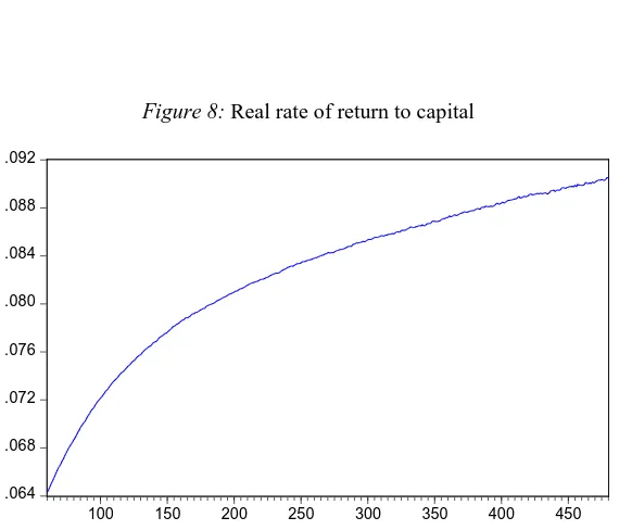
Figure 8: Real rate of return to capital
.064 .068 .072 .076 .080 .084 .088 .092
3
Simulation and results
As pointed out in the introduction of the paper, this study focuses on developing a model that replicates the conjunct dynamics of a financial market, a banking system, and the real economy, mimicking several stylized facts of the latter and grasping, to a certain extent, the implications of banking regulation in economic performance.
Specifically, and based on the model described in Section 2, policy experiments are designed to answer the following seminal questions:
1. Are banks key drivers of economic performance?
2. What effect do different micro-prudential regulations have in economic growth?
3. Are macro-prudential policies effective promoters of financial stability?
In line with the methodology used to calibrate the model (refer to Section 2.3), each experiment encompassed 1000 simulations of 40 years (i.e., 480 time steps).
3.1
The role of banks
From the theoretical standpoint described in Section 1, and following the seminal paper of Diamond and Dybvig (1983), banks play a crucial role in economic growth by pooling liquidity from depositors (who prefer to have their savings placed in liquid instruments) and channeling the funds to firms (who require long-term, large-sum investments in order to generate returns in the future).
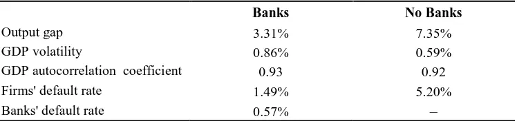
From the results reported in Table 5 it is clear that the existence of banks improves economic development. Indeed, all measures reveal a manifest degradation in median performance when banks are suppressed.
The reason for these phenomena is related with the inner workings of the modelled economy. Since no aggregate equilibrium relationship is forced between the agents’ actual and expected demand, out-of-equilibrium dynamics are created at the level of each specific agent. Since there are no market-clearing mechanisms, the economy spontaneously self-organizes toward a state in which demand persistently exceeds supply. Economic growth in our model is thus a function of the firms’ ability to increase production capacity through investment. The inexistence of banks is a clear obstacle to this process, since in this scenario companies’ investment capacity is limited to their ability to endogenously generate capital. As such, the capacity of the economy to meet aggregate demand is severely hampered when there is no banking system, as reflected in the difference of the output gap (here defined as the difference between potential GDP if all demand was met and actual GDP) in both scenarios (3.31% in the baseline calibration versus 7.35% in the setting with no banks).
This mechanism is also the reason why GDP volatility is less in environments where credit institutions are shut down (0.86% in the baseline calibration against 0.59% in the setting with no banks). The fact that capital investments cannot be leveraged through bank financing means that production responds more slowly to increases in expected demand. Firms adjust more slowly and smoothly to increases in consumption and exports, which in turn reduces GDP’s volatility.
In addition, in our baseline calibration firm failures are mostly attributable to potential gaps between expected and actual demand. These gaps can create an unexpected shock to profits which, associated with firm’s leverage, may render institutions unable to meet their commitments. It would thus be expected that an economy without banks (and thus without credit) would result in lower default rates.
Table 5: Banks vs. no banks
Banks No Banks
Output gap 3.31% 7.35%
GDP volatility 0.86% 0.59%
GDP autocorrelation coefficient 0.93 0.92
Firms' default rate 1.49% 5.20%
Banks' default rate 0.57% –
capital reduces firms’ production capacity to the extent of making them unable to achieve break-even, in which case firms default due to their inability to pay wages. Based on this, it is possible to conclude that banks not only foster growth, they also contribute to the maintenance of the current level of wealth as measured by an economy’s production capacity.
3.2
The impact of micro-prudential policies
The impact of micro-prudential regulation is gauged by considering alternative scenarios in which banks are either riskier or safer than in our baseline calibration. In the risky scenario:
Loan underwriting policies are looser. By imposing a minimum financial autonomy ratio of just 0.3, banks implement lenient credit quality requirements when assessing firms and consumers, thereby significantly increasing the universe of loan-eligible agents;
The required capital adequacy ratio is diminished to just 2%, which significantly increases the capacity of credit institutions to provide loans.
In the safe scenario:
The required capital adequacy ratio is augmented to 15%, a much more credit-constraining scenario than the one imposed in the baseline calibration (8%).
As Table 6 clearly reveals, aggregate macroeconomic performance deteriorates as banks become safer. Indeed, the median output gap is greater in scenarios in which prudential policies are looser (the output gap stands at 3.26% in the risky scenario, which compares to 3.31% in the baseline calibration and 3.66% in the setting with safe banks). This result corroborates our earlier conclusions, according to which increased credit availability improves the creation of value by increasing the speed at which supply is able to meet surges in demand. In the same vein, it is also clear that the mechanisms contributing to GDP volatility are magnified when credit is less constrained.
On the other hand, it is interesting to recognize that the default of firms responds in a non-monotonic way to changes in the micro prudential framework. While the scenario with safe banks displays the highest default rate (1.83%), thus confirming that credit is important for firms to stay afloat in periods of low demand, the scenario with risky banks is not the best performer (the default rate is 0.17% higher than in the baseline calibration). This result suggests that there is an inflection point after which less credit constraints actually contribute to a degradation of firms’ financial robustness. Beyond a certain indebtedness level, and in a manifestation of the financial accelerator effect postulated by Bernanke et al. (1996), increased firm leverage (see Figure 9) makes credit institutions more likely to face distress (due to increased client bankruptcies and credit losses), which in turn increases companies’ likelihood of failure (due to foreclosures by failing banks and credit rationing by low-capitalized institutions).
Table 6: Safe banks, regular banks and risky Banks
Safe banks Regular banks Risky banks
Output gap 3.66% 3.31% 3.26%
GDP volatility 0.74% 0.86% 1.19%
GDP autocorrelation coefficient 0.93 0.93 0.94
Firms' default rate 1.83% 1.49% 1.66%
Figure 9: Credit-to-GDP ratio
(cross-run average)
.1 .2 .3 .4 .5 .6 .7 .8 .9
100 150 200 250 300 350 400 450
Credit-to-GDP - Regular Banks Credit-to-GDP - Risky Banks Credit-to-GDP - Safe Banks
Also remarkable is the fact that firm defaults and the output gap do not move in tandem with each other. Given that new entrants are smaller than incumbent companies, it would be expected that more firm failures would entail decreased economic performance. This thesis is repudiated by the risky scenario, in which the greatest number of defaults coincides with the lowest median output gap. Such a result clearly indicates that firm failures are less likely to slow down the economy when firms have easy access to credit since this source of financing allows entrants to quickly catch up with production requests.
In addition, and despite the fact that bank and firm failures are much more numerous in the risky scenario than in the baseline setting, value-creation improves. This phenomenon stems from the fact that there is an important circuit breaker that prevents the modelled economy from suffering terribly with bank-bankruptcies. The effective resolution of credit institutions, which are terminated immediately upon entering into technical insolvency (i.e., after displaying capital adequacy ratios below 0), means that depositors are not usually bailed-in to a great extent. As such, bank bankruptcies represent salutary events for the economy, which performs better after getting rid of “zombie-banks” that are not able to support investment because they do not comply with micro-prudential requirements.
Important insights can also be drawn from analyzing the behavior of the output gap in time. During the initial stages of the simulations, the gap between production capacity and aggregate demand is large in all scenarios (refer to Figure 10). In the setting with risky banks, the ability of firms to tap external sources of funds is translated into increased leverage and bankruptcies, which in turn contributes to a high output gap when compared to the remaining scenarios. However, as demand grows firms become able to sustain supplementary levels of debt. The output gap is thus closed much more quickly in the scenario in which banks are riskier.
In the long run, growth in the economy is ultimately capped by the growth of consumption and exports. Since the economy does not, on average, experience extraordinary spurs of growth, firms are usually able, in all scenarios and toward the end of the simulations, to raise the necessary capital (either endogenously or through bank financing) to meet demand. As such, the output gaps in different prudential frameworks tend to converge to the same value as time goes by.
Figure 10: Output gap (cross-run average)
.00 .04 .08 .12 .16 .20 .24 .28 .32 .36
100 150 200 250 300 350 400 450
Regular Banks Risky Banks Safe Banks
Figure 11: Firm defaults at each time step (cross-run average)
.0 .1 .2 .3 .4 .5 .6 .7
100 150 200 250 300 350 400 450
Finally, and on micro-prudential policy, it is also relevant to disentangle the effects of changes in the capital framework from modifications to the loan underwriting criteria of banks.
To analyze this, a sensitivity analysis is conducted. Starting from the model’s baseline calibration, we vary, ceteris paribus, the minimum capital requirements of banks and the minimum financial autonomy ratios demanded by credit institutions from their customers. In order to guarantee that the stochastic properties of the model do not affect results, the simulation is performed using the same seed value for the random number generator. Figure 12 and Figure 13 display the differences in the output gap between each scenario and the baseline setting (depicted by the red line).
As can be seen, changes to the capital requirements have a dramatic impact on economic performance. In a clear validation of previous results, it is clear that the output gap is persistently higher (lower) when minimum capital requirements are greater (smaller).
On the other hand, it is also clear that changing the loan underwriting policies has a reduced impact on economic activity. In spite of this, and while there are no relevant differences in median performance between the baseline scenario (median output gap of 2.74%) and the scenario in which the minimum financial autonomy ratio is set at 30% (median output gap of 2.91%), it can be concluded that increasing the strictness of loan underwriting criteria tends to degrade macroeconomic performance (median output gap of 4.09%).
3.3
An exploratory analysis of macro-prudential policies
As already discussed, the recent financial crisis exposed a vicious circle in which difficulties in the banking system can prompt a recession in the real economy that then feeds back onto the financial sector. This phenomenon suggests that banks should increase their capital buffers in periods when systemic risk is greater.
Figure 12: Output gap under varying capital requirements (seed –204145716)
-0.2 0.0 0.2 0.4 0.6 0.8 1.0 1.2
50 100 150 200 250 300 350 400 450
CAR = 0.02 CAR = 0.08 CAR = 0.14
Figure 13: Output gap under varying financial autonomy requirements (seed –204145716)
-.15 -.10 -.05 .00 .05 .10 .15
50 100 150 200 250 300 350 400 450
To test the effectiveness of the counter-cyclical capital buffer, we depart from the baseline scenario by establishing a setting in which the regulator enforces an additional capital surcharge for banks whenever the credit-to-GDP ratio of the economy rises above 35% (which is the average value of the indicator in the baseline cross-run average time series). The buffer is then maintained for at least one year, with the possibility of extension should the economy’s leverage remain above the threshold.
The results reported in Table 7 indicate that imposing a capital buffer of 2.5% (which is the value foreseen in Basel III) or 5% does not have a significant effect on the overall dynamics of the economy. The only visible benefit stemming from this measure is a very mild reduction in the median amount of firm defaults. However, and similarly to the results obtained in the “safe banks” scenario, this is not reflected in persistently lower output gaps (in fact, the opposite occurs).
As explained above, this is underpinned by the fact that firm defaults appear not to have a significant impact on economic growth (in spite of new entrants being smaller than incumbent firms). Indeed, increased access to credit allows new players to quickly catch up with production needs, a phenomenon that can completely offset the slowdown effect of firm bankruptcies.
Table 7: Regular banks and banks subject to macro-prudential policies
GDP autocorrelation coefficient 0.92 0.96 0.93
Firms' default rate 1.43% 1.48% 1.49%
Banks' default rate 0.57% 0.57% 0.57%
3.4
Endogenizing bank failures
As described above, bank failures are a beneficial phenomenon in our baseline model. A bank that enters into resolution is naturally not complying with minimum capital requirements and is thus not allowed to make new loans. The assumption that this agent can be replaced by foreign investment by a credit institution that can finance economic activity from the outset could be one of the reasons why our model reveals improved economic performance with risky banks.
To address this shortcoming, we endogenize the cost of bank failures. As before, depositors of failed banks are still bailed-in, thus absorbing the losses of the institution and raising its capital to zero. Under the new setting, however, depositors further see a part of their deposits being converted into equity so that the new institution complies with minimum capital requirements (specifically, the capital adequacy ratio is set at 12% in excess of the minimum in each scenario). Because bank recapitalization costs are now fully borne by depositors, the amount of cash available for agents to consume (in the case of consumers) and invest (in the case of firms) is reduced. The consequences of a bank failure for the economy are thus magnified in this setting.