The purpose of this research is to analyze and test the effect of customer loyalty on consumer credit profitability. Loyalty Index Score was developed to determine the level of customers’ loyalty level through 4 main variables; Longevity, Depth, Breadth and Referrals. The effect of Loyalty Index Score on profitability was further tested by path analysis to find out the significance direct relationship between loyalty and profitablity and the indirect relationship between the two variable through bucket. The result showed that loyalty has a significant effect on profitability either directly or indirectly. It was concluded that direct loyalty effect on profitability is lower than that of the indirect effect through bucket. The conclusion could be made by analyzing the available data from personal loan customers in one of the biggest multinational bank in indonesia during October 2010 until March 2011.
© 2012 IRJBS, All rights reserved. Received: September 10, 2011
Final revision: February 8, 2012
Keywords: Loyalty, Consumer Credit, Credit Risk, Profit, Path Analysis
Corresponding author: * galihprihartono@yahoo.com ** sumarwan@mb.ipb.ac.id *** achsani@yahoo.com **** koko_kir@yahoo.com
Aditya Galih Prihartono
*, Ujang Sumarwan
**, Noer Azam Achsani
***,
Kirbrandoko
**** Institut Pertanian Bogor, BogorA R T I C L E I N F O A B S T R A C T
A
s stated by Jacoby and Chestnut (1978), loyalty can be measured through the behavioral approach, attitudinal approach and composite approach. The behavioral approach is based on consumers’ actual or reported purchasing behavior and has often been operationally characterized as sequence of purchase, proportion of purchase, and probability of purchase. However, this approach has beencriticized by Dick and Basu (1994) as lacking a conceptual standpoint, and producing only the static outcome of a dynamic process. In addition, Pritchard and Howard (1997) also state that focusing on behavior alone cannot capture the reasons behind the purchases: repeat purchase may occur simply for arbitrary reasons such as price, time convenience and lack of choice, other than from any sense of loyalty or allegiance.
Vol. 5 | No. 1 ISSN: 2089-6271
The Significance of Loyalty
In the attitudinal approach, based on consumer brand preferences over time or purchase intentions, loyalty reflects consumers’ psychological commitment to a brand, and is studied via its dimensions such as repurchasing intentions, word of mouth referrals, complaining behavior (Jones and Sasser, 1995; de Ruyter and Bloemer, 1998). The attitudinal measure explains an additional portion of unexplained variance that behavioral approaches do not address (Backman and Crompton, 1991). However, study attitude alone cannot determine competitive effects, familiarity, and situational factors (Baloglu, 2002).
In practical research, comparing between beha-vioural and attitudinal approach, behavioral mea-sures are a common approach to operationalize loyalty, due to the difficulties in measuring attitu-dinal loyalty. As suggested by Opperman (2000) behavioral measures will be much better than atti-tude measures because measuring attiatti-tudes over a longer time period is in most cases impractical.
Parasuraman, Zeithmal and Berry (1994) developed a loyalty scale including dimensions such as loyalty to company, propensity to switch, willingness to pay more, external and internal response to problem. Some researchers (Taylor, 1998; Yoon and Uysal, 2003) measured consumer loyalty with three indicators: 1) likelihood to recommend a product or service to other; 2) likelihood to purchase a product or service again; and 3) overall satisfaction/feeling. Hepworth and Mateus (1994) adopted similar indices to assess loyalty, including intention to buy same product,
intention to buy more product, and willingness to recommend the product to other consumers. As can be understood from the loyalty development principle in these researches, loyalty has been measured in the mixed way from both behavior apprach and attitude approach, or in simple term called the composite approach.
More recently, It has been argued that customer loyalty is a multidimensional concept including both behavioral element (repeat purchases) and attitudinal element (commitment) and the use of composite measure increases the predictive power of the construct, as each variable cross-validates the nature of truly loyal relationship (Dick and Basu, 1994). However, this approach has limitations because not all the weighting or quantified scores may apply to both the behavioral and attitudinal components, which may have different measurements.
Classifying Loyalty
Backman & Crompton (1991) explained four loyalty types based on the cross classification of consumers’ behavioral consistency (behavior) and psychological attachment (attitude): low loyalty, spurious loyalty, latent loyalty, and high loyalty. While empirical support for the typology has been noted in wider marketing literature (Dick and Basu, 1994), and leisure services (Selin et al. 1988, Backman and Crompton 1991), hospitality researchers have further confirmed the application of four distinct types of loyalty in a multitude of settings (Baloglu, 2001; Pritchard and Howard, 1997).
Attitude
Low High
Behaviour
High Spurious Loyalty True Loyalty
Low Low Loyalty Latent Loyalty
Table 1. Loyalty Typology
Source: Backman & Crompton (1991)
As can be seen from table 1 , there are 4 major loyalty typology in regards to its attitude and behaviour level. The definition is as follow:
• True/high loyalty customers are characterized by strong attitudinal attachment and high behavioral patronage with a product/service, and are least vulnerable to competitive offerings.
• Latent loyalty customers are those who show low patronage levels in spite of a strong attitudinal attachment to the brand. This may occur because patronage barriers such as price, convenience (e. g., times available, routing), or location (e. g., ease of access, distribution) prevent them from becoming repeat customers.
• Spurious/artificial loyalty customers are those who make frequent purchases yet are not emotionally attached to the brand. The high patronage level of spuriously loyal customers may be attributed to habitual buying, financial incentives, convenience, lack of alternatives, etc.
• Low loyalty customers refer to those exhibiting low levels of both attitudinal attachment and behavioral usage with a brand. Spurious- and low-loyalty groups are more susceptible to ‘courting’ from competitors, as their patronage tends to be highly volatile.
This typology gives another hints that actually each customer has a different loyalty level and its influence to profitability cannot be doubted (Oliver 1997; Hallowel 1996). More information can be elaborated mainly to see the loyalty level of a customer into profitability which can be inferred either directly and indirectly through share of wallet, market share, and revenue received.
Loyalty in Consumer Credit
In consumer credit scenario, loyalty strategy has been developed by money lenders or banks. Eakuru & Mat (2008) found that to increase loyalty, trust and image is two among many other things to be considered. This is to ensure the existence
of long term relationship between money lender and its customer. The common strategy in current practice are as follow:
• Point reward to be traded in with direct prize • Point reward to be converted with lucky dip • Direct discount for credit card purchase • Sales offering with special discount • Cash Back
• Special card discount • Buy 1 get 2
In an indirect way, some loyalty strategy also can be listed as follow:
• Cross sell with non loan products such as insurance, savings account.
• Cross sell with other credit cards brand within the same bank provider
• Cross sell with unsecured personal installment loan
• Simplification strategy, 1 bill under 1 credit card
• Balance transfer
As if customer take the products as listed above within one bank, it is expected that customer will keep loyal to that bank and in the end will produce long term relationship. Customer will think twice before reducing or terminating its financial relationship with the bank because of that dependency. However, since this is a consumer credit products with some credit risk involved, there are some critical factors to be considered such as customer capacity to pay and character. Customer character might be easier to check from past historical credit performance (for those who already have credit performance) however the story might be different for capacity to pay. Capacity to pay will be depends on customer current condition which may very different from the beginning.
(e.g. age and income) rather than resulting from a positive attitude towards their bank. This means, no matter how loyal the customer is, when there is income (or capacity to pay) issue in customer financial cycle, profitability will be at risk. in the end, there will be priority to be chosen by the customer which one to be taken care in the first place, which products above the other.
Payment Default
Payment default in credit scenario will happen when customer cannot repay the installment on the agreed date. This condition can happen due to so many reasons. Ford (1990) list down some of the reasons as follow:
• Unemployment
• The rising levels of divorce and relationship breakdown
• The growth of low wage, less secure work • Illness
• Rising costs (involuntary increases such as interest rate increases, rental increases, etc) • Over commitment to credit (reinforced by
sophisticated marketing and relaxation of controls on lending)
Lyons (2001) explains more detailed information regarding household capability to repay its loan:
1. Favorable economic conditions – rising
employment level and a dramatic rise in stock and bond prices have resulted in increases in both personal income and overall wealth providing household with a greater ability and incentive to spend. The recent expansion has not only encouraged households to take on additional debt, but also to shift into a greater share of their liquid assets, which act as a buffer against unexpected changes in income, into more illiquid financial instruments.
2. Unanticipated life disruptions – Divorce, job
loss, and health problems are also cited as likely contributors to household repayment problems. Unanticipated events such as divorce often result in a significant drop in household income. As a result, households
may be unable to repay their debt simply because they are poor. It may also be the case that household may run into financial problems because they are overextended. A significant drop in income coupled with severe indebtness may result in a household’s inability to repay its debt.
3. Household debt burden – both the incidence
of debt and the amount of debt held by households have risen dramatically over the last twenty years. In particular, households have seen large increases in consumer debt. A higher proportion of credit users and a more intensive use of credit have resulted in dramatically higher debt to disposable income ratio and higher ratio of debt payment to income. However, these findings are based on aggregate numbers. The effect of greater debt burden on household repayment problem depends on substantially upon which household have taken on additional debt and the distribution of that debt. It may be that a substantial fraction of the households with large debt to income ratios also have substantially large asset holdings. In this case, debt burdens may not be a significant contributor to the rise in repayment problems after asset holdings are taken into account.
4. Changing attitudes towards credit usage,
delinquency – it is important to keep in mind that the recent rise in delinquencies may also be due not to an increase in debt problems per se but to a change in how individuals choose to deal with these problems. Greater social acceptability of indebtness coupled with a diminishment in the social stigma associated with bankruptcy may have resulted in an increase in financial irresponsibility and a rise in the willingness of households to declare bankruptcy.
5. The democratization of credit – since 1980’s,
the credit industry has made a number of effort to provide additional and more affordable Liquidity to households traditionally constrained by the credit markets. Households
have seen lower interest rates, fees and down payment, more flexible underwriting standards, and new financial instruments and expanded product offerings. Over this time period, the credit industry also engaged in more aggressive marketing strategies. Increased profitability within the credit industry has led to an in surge of new lenders willing to take on more risky (marginal) borrower and an additional increase in the supply of credit to those traditionally constrained. While recent financial developments have made it easier for traditionally constrained households to obtain credit, they have also raise concerns that these innovations have made it easier for such household to live beyond their means. For this reason, many researchers have argued that the recent democratization of credit has likely contributed significantly to the rise in delinquencies.
Conclusion could be made based on both explanations above are as follow:
• Capacity to pay issue may come as a result of decreasing of income due to unexpected event such as divorce, unemployment, sickness.
• On the other side, capacity to pay issue may also come as a result of increasing expense more than income. This can happen due to lack of control in financial budget, lifestyles, increasing living cost.
Hence, the combination of both expense and income determine how much disposable income left to ensure that the customer can pay its loan every month.
Buckets
In general, the risk level of debtors in a portfolio may vary from one to another. To differentiate this, the debtor is grouped into their product type. Depends on its rule and regulations for each company and country, product type is determined mainly by some key points based on (Finlay 2008):
1. Whether credit is provided on a secured or
unsecured basis.
2. Whether repayments are amortizing or
balloon.
3. Whether the credit agreement is fixed sum or
running account.
4. Whether credit is provided on a restricted or
unrestricted basis.
5. Whether credit is provided on a credit sale,
conditional sale or hirepurchase basis (for restricted credit only).
6. Whether the credit agreement is a
debtor-cre-ditor or a debtor-credebtor-cre-ditorsupplier agreement.
7. The amount of credit available. 8. The term (duration) of the agreement.
9. The cost of credit. If several different charges
are applied, then each of these can be considered to be a separate sub-feature of the product.
The product type determines which accounting princples to be followed especially related to revenue and credit loss recognition. A credit card product will have a different rule with a mortgage product due to its risk level. The difference commonly can be seen on the timing of when the accounts will be written off or how long the days past due to be decided in a portfolio or product. In general, here are some common market practice (Smith and Jin, 2007):
• 120 days past due: this is commonly used for unsecured – close end products or in many terms called personal loan. The accounts will be categorized as write off when it reach 120 days pas due. with 30 days segregation, it means there are 4 buckets used to measure portfolio quality (120 dpd ÷ 30 days = 4). • 180 days past due: this is commonly used for
unsecured – open end products or in many terms called credit card. The acounts will be written off when it reach 180 days pas due. with 180 days past due, there are 6 buckets used to measure portfolio quality (180 ÷ 30 days = 6).
for secured – close end products or in many terms called mortgage. The accounts will be written off when it reach 720 days past due. It means there are 24 buckets used to measure portfolio quality (720 ÷ 30 days = 24). However, in a normal circumstances, bank will prefer to sell the asset and do the write down to minimize its loss. Write down is an activity to re-evaluate asset’s value according to market value. If the asset is a property or land, commonly its value will be higher than its first valuation.
To simplify the operational and strategy used in risk management, the customers will be grouped into its bucket. Bucket will be determine by its days past due, how many days the customers missed their payment. The higher the days pas due, the closer it is to the credit loss numbers which in the end will reduce profitability. Below figure 1 shows an example of this concept (Lawver, 1993).
In real situation service level is also correlated inline with the days past due numbers. Obviously, the highest service level can be seen when the customer stay current, always pay their installment or minimum payment and along with higher days past due, lower service level will be felt by the customer. This is for a simple reason, the money lender will focus on getting the payment to save their asset in the first place rather than serving the customer needs. The trust level for both parties (customer and money lender) will be at risk because both parties has a different interest and
Figure 1. Buckets (Level of Delinquency)
priority. Hence, there is a point along the days past due line where customer payment is the only thing matter. This is where Risk mitigation play a big part, to give more alternative options for the customer in making their payment, most of it in terms of payment discount or delayed payment with schedule.
Profitability and its Relationship with Loyalty
There were many previous research which relates between Loyalty and Profitability. One of which was done by Hallowell (1996) who illustrates the relationship of profitability to intermediate, customer-related outcomes that managers can influence directly. The result of this research shows that Path analysis performed on measures of customer satisfaction, loyalty, and profitability was inconclusive. The analysis neither confirmed nor denied that the relationship path hypothesized by the service management literature (customer satisfaction --> customer loyalty --> profitability) is stronger than a direct customer satisfaction --> profitability relationship. Another research by Reicheld, Markey and Hopton (2000) and Oliver (1997) shows the relationship between loyalty and profit. Even though the measurement was made at the high level, it was confirmed that loyalty significantly influence profitability mainly in a long term perspective.
In addition, It has been estimated that it costs five times as much to attract a new customer as it does to retain a existing one, according to research by the American management Association (Kotler, 1994;
Peppers & Rogers, 1996) and this relationship is particularly obvious in the services sector (Ennew & Binks, 1996). Therefore, company understand the importance of developing a good close relationship with existing and new customers. Instead of attracting new customers, they would like to perform as well as possible more business operations for customers in order to keep existing customers and build up long-term customer relationship. Based on this reason, loyalty as the basis of long term relationship requirements, needs to be focused on. It wil need customer value analysis to understand about their customers, to retain valuable customers and finally to bring plenty of profits for themselves.
Customer value analysis is a kind of analytic method for discovering customers’ characteristics and makes a further analysis of specific customers to abstract useful knowledge from large data. Thus, it is clear that company apply value analysis method to customers for knowing about who are the target customers which contribution is outstanding. Kaymak (2001) pointed out that the RFM model (Recency, Frequency and Monetary) is one of the well-known customer value analysis methods. Its advantage is to extract characteristics of customers by using fewer criterions (a three-dimension) as cluster attributes so that reduce the complexity of model of customer value analysis. Moreover, from view of the consuming behavior, Schijns and Schroder (1996) also supported that the RFM model is a long-familiar method to measure the strength of customer relationship. Retention cost is far less costly than acquisition cost (Kotler, 1994; Peppers & Rogers, 1996), therefore, company are intent via using RFM analysis to mine databases for knowing about customers who spend the most money and create the biggest value for company.
The RFM analytic model is proposed by Hughes (1994), and it is a model that differentiates important customers from large data by three variables (attributes), i.e., interval of customer
consumption, frequency and money amount. The detail definitions of RFM model are described as follows:
1) Recency of the last purchase (R). R represents recency, which refers to the interval between the time that the latest consuming behavior happens and present. The shorter the interval is, the bigger R is.
2) Frequency of the purchases (F). F represents frequency, which refers to the number of transactions in a particular period, for example, two times of one year, two times of one quarter or two times of one month. The many the frequency is, the bigger F is.
3) Monetary value of the purchases (M). M represents monetary, which refers to consumption money amount in a particular period. The much the monetary is, the bigger M is.
According to the literature (Wu & Lin, 2005), researches showed that the bigger the value of R and F is, the more likely the corresponding customers are to produce a new trade with company. Moreover, the bigger M is, the more likely the corresponding customers are to buy products or services with company again. Newell (1997) added that RFM method is very effective attributes for customer segmentation.
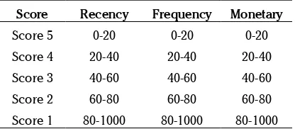
Cheng & Chen (2009) proposed a practical approach on segregating the typology of loyalty into 5 level (score 1 to 5) the score will be given to the accounts based on its Recency, Frequency and Monetary by dividing the overall sample into 20% for each level.
Score Recency Frequency Monetary
Score 5 0-20 0-20 0-20
Score 4 20-40 20-40 20-40
Score 3 40-60 40-60 40-60
Score 2 60-80 60-80 60-80
Score 1 80-1000 80-1000 80-1000
Since composition of sample cannot be determined at the time of the proposal was made, this approach is quite practical and simple to be followed.
Furthermore, in the same research, Cheng and Chen (2009) also propose another approach on scoring design. This second approach was made by first determining the criteria of each segment to be scored. This approach is possible whenever there is huge sample to be used and therefore it can avoid empty segment with no sample at all.
Score ScalingName Recency Freq. Monetary
Score 5 Very High 1 month 25 1000
Score 4 High 3 month 20 7000
Score 3 Medium 6 month 15 4000
Score 2 Low 9 month 10 2000
Score 1 very low 12 month 1 1000
Table 3. RFM Scaling 2
Whatever approach to be used, the basic foundation is to ensure that all segment in the loyalty class should be avaliable and cannot be left blank. Hence, the approach should be flexibel enough to cater the end state of the research.
METHODS Data Collection
This research was done in one of multinational banks in Indonesia from October 2010 – March 2011. Location of research will cover Jakarta, Bandung, and Surabaya. Research was conducted by using descriptive analytical methods to describe processes and phenomena that occur through a
quantitative approach based on past historical records for each customer in the sample.
Data for this research came from 2 types, primary and secondary. Primary data was taken from internal database, past historical records. Secondary data was collected from internal company and other related sources such as previous research, newspaper, Bank of Indonesia. Sampling for this research was done by stratified simple random sampling from list of customers in Bank A. Sampling technique details can be seen as follow:
• Sampling Element: Bank’s Customer
• Population: All Personal Loan customer at Bank X ( around 100,000)
• Sampling Unit: Customer who is still registered as Personal Loan customer in Bank X with minimum Months on Book (MOB) of 1 year (12 months).
• Sampling Frame: Non Delinquent Customer and Delinquent Customer (>30 DPD)
• Sampling Size: 31700
• Sampling procedures: Sampling will be done by classifying the population into 4 groups (Non Delinquent – Normal Capacity to pay, and Delinquent – Non Normal Capacity to pay: Early delinquent, Late delinquent and Restructuring accounts). Sample will be taken randomly from all groups to be further processed to the next step.
Conceptual Framework & Hypothesis
The conceptual framework in this research can be illustrated in figure 2.
From figure 2, the main conceptual framework in this research is Loyalty, Buckets and Profitability. Loyalty will be measured by 4 indicators: Longevity, Breadth, Depth and Referrals where all of this indicators will be blended and converted into a single score as overall Loyalty Score. Loyalty Score will be used as independent variable to profitability.
Buckets will be directly known by the days past due. This information will be collected directly from customer historical records in the system. As explained in the earlier section, bucket 0 means that customer is non delinquent, bucket 1, customer is in 30 days past due, bucket 2 is 60 days past due and so on.
Profitability measurement will be done through payment tracking which was made by the customers within a particular period. The payment will show whether or not it can save the accounts from further flowing to the next bucket (balance saved) and at the same time, whether or not the payment can cover the interest and fees (revenue collected). Based on this explanation, there are 2 hypothesis in this paper:
H1: There is significant effect of Loyalty & Bucket to Profitability
H2: There is significant effect of Loyalty to Buckets
Analysis Tools
In the beginning, demographic analysis will be analyzed to give hints on data distribution based on customer basic information such as age, marital status, dependence, income group, gender, education and last status. The next step is to develop the basic criteria, what range to be used in each 4 Loyalty indicators (longevity, depth, breadth, referrals). To determine this range, central tendency value will be calculated (mean, median, mode, max and min) where those value will be used as basic reference in determining the score range. Once determined, data normality
analysis will be the next step to be done. In here, we will see some basic information such as skewness, kurtosis and standard deviation. This step is needed to confirm data normality before proceeding to the next step.
Following the above analysis, path analysis wil be done from loyalty to buckets and loyalty & bucket to profitability. From there we will see beta and regression numbers whether or not each path has a significant value. Based on this information, we will then analyze the direct and indirect effect of loyalty to profitability. The ability of path analysis to decompose the correlation between any two variables into a sum of simple and compound paths yields information about casual processes, which provides a more explicit approach for the explanation of the relationships under investigation (Ullman, 1996; Yang and Trewn, 2004; Kumar et al. 2008)
RESULTS AND DISCUSSION Demography Analysis
In overall, there were 31,700 accounts sample from total around 100,000 populations. In path analysis and structural equation modelling as a rule of thumb, any number above 200 (critical sample size) is understood to provide sufficient statistical power for data analysis (Hoelter, 1983; Hoe, 2008). The sample 31,700 is considered as more than enough to explain the overall information. The sample was chosen after considering sample representativeness in each bucket segment, missing value and general requirements as stated in the methodology section.
As can be seen on Table 4, it shows sample distribution across 7 demography items. It shows the total samples for each demography items with its cumulative numbers.
From total 31,700 samples, Male customer (61.82%) seems to be higher than Female (38.18%). This is a normal situation because commonly the one who work for the family is Male than Female and hence,
Loyalty Score Profitability
Buckets
Items N % Cummulative % Cummulative
1. Gender 31,700
Male 19,596 61.82% 19,596 61.82%
Female 12,104 38.18% 31,700 100.00%
2. Dependence 31,700
0 12,731 40.16% 12,731 40.16%
1 4,952 15.62% 17,683 55.78%
2 6,982 22.03% 24,665 77.81%
3 4,725 14.91% 29,390 92.71%
4 1,667 5.26% 31,057 97.97%
>4 643 2.03% 31,700 100.00%
3. Marital Status 31,700
Married 26,466 83.49% 26,466 83.49%
Single 5,234 16.51% 31,700 100.00%
4. Education 31,700
<S1 13,945 43.99% 13,945 43.99%
S1 16,995 53.61% 30,940 97.60%
>S1 760 2.40% 31,700 100.00%
5. House Status 31,700
Sewa 5,282 16.66% 5,282 16.66%
Keluarga 10,566 33.33% 15,848 49.99%
Sendiri 15,852 50.01% 31,700 100.00%
6. Monthly Income 31,700
<5 Juta 11,977 37.78% 11,977 37.78%
<10 Juta 6,050 19.09% 18,027 56.87%
<25 Juta 5,161 16.28% 23,188 73.15%
<50 Juta 2,889 9.11% 26,077 82.26%
>=50 Juta 5,623 17.74% 31,700 100.00%
7. Age 31,700
<30 5,286 16.68% 5,286 16.68%
<40 13,522 42.66% 18,808 59.33%
<50 9,084 28.66% 27,892 87.99%
>=50 3,808 12.01% 31,700 100.00%
Figure 2. Conceptual Framework
has monthly income less than Rp 5 million per month while other income segments were 19.09%, 16.28%, 9.11% and 17.74% respectively for <10 million, <25 million, <50million and >= 50 million. In addition to this, from age point of view, customer with age range 30 – 39 years dominates the total distribution at 42.66% followed by 40 – 49 years (28.66%), 20 – 29 years (16.68%) and >= 50 years (12.01%).
Based on the above explanation, in summary, sample distribution is dominated by male customer, married, no dependence, has Bachelor degree, income below 5 million, age 30 – 39 years and owned the house. This is a typical of low to mid
level of customer segment which can be someone who just started their job (but not a fresh graduate) and family, need the cash to strengthen their future plan either short or long term. Normally, this segment is not price sensitive but more into cash flow sensitive or in other words, very sensitive to the total installment that they need to pay on a monthly basis.
Longevity
Longevity in credit management terminalogy is equal to Month On Book (MOB). MOB starts when banks disburse the credit to the customer’s account. Table 5 shows the Longevity distribution across all samples.
it shows higher proportion in the sample. In term of Marital Status, Married couple dominates the total sample with 83.49% while Single customers were below 17%. The sample distribution from total dependence view were quite dominated by zero (0) dependence followed by 2, 1, 3, 4 and >4 respectively at 40.16%, 22.03%, 15.62%, 14.91%, 5.26%, 2.03%.
Based on highest education level, customer with Undergraduate or Bachelor (S1) degree reach more than 50% followed by below Undergraduate degree at almost 44% (Diploma, High School,
Junior High School) and finally those customers with more than education level equal to or more than Graduate or Master Degree at 2.40%. On the other items, House ownership status, customer who owned the house contributes to 50% of the total samples while living with family reach the second rank at 33% and renting the house in the bottom place at 16.6%.
Monthly income as one of key drivers in determining total credit to be given is also part of this demography analysis. As can be seen on Table 4.1, the sample shows that 37% of total distribution
Longevity Total % Cummulative Cummulative%
12 48 0.15% 48 0.15%
13 2,229 7.03% 2,277 7.18%
14 1,797 5.67% 4,074 12.85%
15 2,531 7.98% 6,605 20.84%
16 2,332 7.36% 8,937 28.19%
17 2,356 7.43% 11,293 35.62%
18 2,263 7.14% 13,556 42.76%
19 2,140 6.75% 15,696 49.51%
20 2,042 6.44% 17,738 55.96%
21 1,995 6.29% 19,733 62.25%
22 2,039 6.43% 21,772 68.68%
23 1,511 4.77% 23,283 73.45%
24 1,642 5.18% 24,925 78.63%
25 1,479 4.67% 26,404 83.29%
26 1,164 3.67% 27,568 86.97%
27 1,554 4.90% 29,122 91.87%
28 1,212 3.82% 30,334 95.69%
29 1,347 4.25% 31,681 99.94%
30 9 0.03% 31,690 99.97%
31 10 0.03% 31,700 100.00%
Grand Total 31,700
Max 31
Min 12
Mean 20
Median 20
Mode 15
As shown on table 5, accounts sample were distributed with MOB 12 (the lowest) and MOB 31 (the highest). The average MOB were 20 with the same Median numbers which means that the accounts sample is quite focus at the center value, and at the same time with Mode value were 15, lower than Mean and Median value. This value will be used as the basis to determine the cut off score for Longevity criteria from the lowest till the highest. Table 6 is the summary of the score distribution after considering Max, Min, Mean, Median and Mode value in Longevity variable.
The Mean and Median which has the same value at 20 MOB, will get 30 points while Max and Min number will get 10 points and 50 points respectively for MOB <14 and >=30. Easily we can determine the score of 20 and 40 is somewhere in between those criterium above. By looking at data distribution, it is proposed to give 20 points for MOB <15 and 40 points for MOB <30. By using the above criterium, half of the sample were distributed at 40 points followed by 30, 10, 20 and 50 points.
Depth
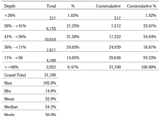
Depth is the second variable in Loyalty Index Score development. Depth itself can be defined as total monetary amount or frequency payment has been made by the customer to the bank as compared to the total monetary amount or tenure that they need to pay till the last installment. Depth numbers will be converted into a percentage number which shows the level of loan completion from beginning
till the end. A customer who has paid the loan installment for 18 months in a 36 months total tenure will have 50% of depth value (18/36 = 50%). The detail distribution can be seen in Table 7.
Table 7 shows data distribution in Depth category. Using the same approach with Longevity category, 30 points will be given to the midlle value 56% (with Mean 55.9% and Median 54.2%), while 10 points and 50 points will be given to those value at the range of Min and Max numbers (14.6% and 105%) respectively. The cut off for 20 points will be given to the range of 36% - 56%. The criteria cut off at 36% is used as the mid point between the lowest depth % (14.6%) and the mean dept % (56%). On the other side, cut off at 91% is used due to more as judgemental approach to differentiate those who will finish the loan versus those who still below 90%. Based on that, 40 poiints will be given to the range of 56% - <91% and 50 points will be given to those customer with Depth value euqal or more than 91%.
Based on the above arrangement, Depth score distribution can be seen on Table 8.
By looking at Depth Score distribution, 41.07% of sample distribution were under 56% - <91% which means the customer had paid their installment more than a half from total tenure. The next portions were those customers with score 20 and 30 which means ranging from 36% - 56%. The last one will be those <36% with 12.85% and >=91% with 4.28%.
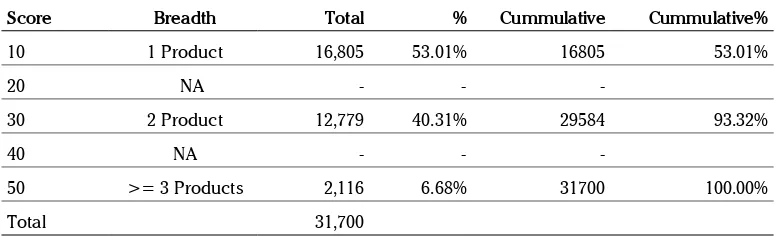
Breadth
Breadth is the total products which was enjoyed or bought by the customer. Based on data collections, we are able to identify 3 other products which the customer may have besides personal loan product that they keep at the moment. The other 3 products were Credit Card, Credit Guard Insurance and Life Protector Insurance. Credit Card is a credit revolving product, a very common consumer credit products. Credit Guard Insurance is an insurance product to cover customer’s personal
loan product in case they cannot pay the loan due to illness and death. Life Protector Insurance is an insurance product to cover cutsomer’s life, a very common life insurance product as we know. Sample distribution based on breadth category is as shown in Table 9.
Accounts distribution under breadth category were 53% customer hold 1 product, 40.31% enjoy 2 products and 6.68% has 3 products in hand. Using slightly modified approach, score cut off were
Score Longevity Total % Cummulative Cummulative%
10 <14 2,277 7.18% 2,277 7.18%
20 14 - <15 1,797 5.67% 4,074 12.85%
30 15 - <20 11,622 36.66% 15,696 49.51%
40 20 - <30 15,985 50.43% 31,681 99.94%
50 >=30 19 0.06% 31,700 100.00%
Total 31,700
Table 6. Longevity Score Distribution
Depth Total % Cummulative Cummulative %
<26% 577 1.82% 577 1.82%
26% - <41% 6,735 21.25% 7,312 23.07%
41% - <56% 10,010 31.58% 17,322 54.64%
56% - <71% 7,617 24.03% 24,939 78.67%
71% - <86 4,709 14.85% 29,648 93.53%
>=86% 2,052 6.47% 31,700 100.00%
Grand Total 31,700
Max 105.0%
Min 14.6%
Mean 55.9%
Median 54.2%
Mode 50.0%
Table 7. Dept Distribution
Table 8. Depth Score Distribution
Score Depth Total % Cummulative Cummulative%
10 <36% 4,073 0 4,073 12.85%
20 36% - <46% 6,841 0 10,914 34.43%
30 46% - <56% 6,408 0 17,322 54.64%
40 56% - <91% 13,020 0 30,342 95.72%
50 >=91% 1,358 0 31,700 100.00%
Table 9. Breadth Distribution Table 11. Referral Distribution
Breadth Total % Cummulative Cummulative %
1 16,805 53.01% 16,805 53.01%
2 12,779 40.31% 29,584 93.32%
3 2,116 6.68% 31,700 100.00%
Grand Total 31,700
Max 3.0
Min 1.0
Mean 1.5
Median 1.0
Mode 1.0
determined based on its Max, Min and Mean value. Due to max number of products in hand stop at 3 products, we can conclude that 10 points will be given to those customer with 1 product, 30 points for those who hold 2 products and 50 points to those who have 3 products in hand. This approach are inline with the first 2 category, Longevity and Depth.
After scoring all sample, Table 10 shows the Breadth Score Distribution with its cummulative value.
The score distribution is inline with Breadth raw data distribution with 53%% sample get 10 points, 40.31% sample get 30 points and 6.68% sample get the maximum 50 points.
Referral
The last category in Loyalty Index Score development is called Referral. Referral is the total accounts which was referred by the existing customer to also enjoy the products that they enjoy. This is one of the so called active Loyalty concept where the customer reccomend the product to other people. In consumer credit term, this is called Member Get Member program (MGM) and most of the time, customer who did this is the best customer in the portfolio. They are the one who speak positively about the products and help the company to get free advertisement from them. Referral data distribution can be seen in Table 11.
From total samples, it was found that 28.45% referred this personal loan product to another 1 customer. Less than 0.5% referred more than
Score Breadth Total % Cummulative Cummulative%
10 1 Product 16,805 53.01% 16805 53.01%
20 NA - - -
30 2 Product 12,779 40.31% 29584 93.32%
40 NA - - -
50 >= 3 Products 2,116 6.68% 31700 100.00%
Total 31,700
Table 10. Breadth Score Distribution
Referral Total % Cummulative Cummulative %
0 22,669 71.51% 22,669 71.51%
1 9,020 28.45% 31,689 99.97%
2 9 0.03% 31,698 99.99%
3 1 0.00% 31,699 100.00%
9 1 0.00% 31,700 100.00%
Grand Total 31,700
Max 9.00
Min 0.00
Mean 0.29
Median 0.00
Mode 0.00
1 while the other 71.51% had never referred the accounts to the other potential customer. This can be, referral was in place but the applications was rejected by the bank due to many reasons.
Scoring approach for this category was done by direct simple approach i.e. 0 points for no referral, 10 points for 1 referral, 20 points for 2 referrals, 30 points for 3 referrals, 40 points for 4 referrals and 50 points for 5 referrals and more. This approach is choosed becasue there is no difference in median and minimum value on referals while maximum value reach 9 referrals. Hence, the scoring cirterium was made based on simplicity practical used only.
The scoring result by using the above criterium under Referrals category are as shown in Table 12.
The scoring distribution under Referral category is dominated by 0 referral and it is followed by 1 referral. The main difference in scoring approach for Referral category as compared to the other 3 is 0 (zero) score point for those who never refer the products to the other customer up till the acocunt is booked. There was also no 40 points given as a result of no total referral that equal to 4 accounts.
Overall Scaling
The last four section describes about LIS development, distribution and its scaling. To summarize and ease of overall understanding, Table 13. shows the summary of Score level and scaling per LIS indicators.
As summarize on Table 3.9, the same approach had been used by Cheng and Chen (2009). Scaling
Score Referral Total % Cummulative Cummulative%
0 0 22,670 71.51% 22670 71.51%
10 1 9,019 28.45% 31689 99.97%
20 2 9 0.03% 31698 99.99%
30 3 1 0.00% 31699 100.00%
40 4
50 >=5 1 0.00% 31700 100.00%
Total 31,700
Score Longevity Referral Depth Breadth
0 NA 0 NA NA
10 <14 1 <36% 1 Product
20 14 - <15 2 36% - <46% NA
30 15 - <20 3 46% - <56% 2 Products
40 20 - <30 4 56% - <91% NA
50 >=30 >=5 >=91% >= 3 Products
Table 13. Summary of LIS Scaling
for each indicator was done by specific criteria, considering central tendency value for each indicator. Score 0 (zero) was applied only for Referrals, while Breadth did not have Score 20 and 40. The rest of score level had been applied to all scaling.
Combination of score from each indicator shows the total Loyalty level of each account in the sample. It is one from so many ways to predict customer’s loyalty level and therefore, it can be used to further check its impact to profitability on all or specific segment.
The Development of Loyalty Index Score
Loyalty Index Score (LIS) is the sum score of the 4 Loyalty indicators as explained in the earlier section. The score from all indicators (Longevity, Depth, Breadth and Referral) will be added to get
one single score as LIS. LIS is the combination and mix from all indicators to show customer’s loyalty level towards the products offered, in this case personal loan product. In simple term, LIS model is as follow:
Loyalty Index Score = Longevity + Depth + Breadth + Referral
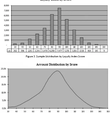
LIS will be tested further, whether it can influence profitability level of a portfolio through 2 combination, credit loss and revenue. However, before going into further, we will need to asses data normality after all score is added and become LIS. Table 14. shows the sample distribution by LIS. Figure 3 and 4 shows the spread of data from the lowest score into the highest one. It can be seen clearly that the data composition has a good shape which indicate a normal distribution curve. Table 14 Sample Distribution by Loyalty Index Score
LIS Grand Total % Cummulative Cummulative %
30 262 0.83 262 0.83
40 396 1.25 658 2.08
50 1261 3.98 1919 6.05
60 2241 7.07 4160 13.12
70 3470 10.95 7630 24.07
80 6200 19.56 13830 43.63
90 7477 23.59 21307 67.21
100 5176 16.33 26483 83.54
110 3061 9.66 29544 93.20
120 1538 4.85 31082 98.05
130 464 1.46 31546 99.51
140 145 0.46 31691 99.97
150 9 0.03 31700 100.00
Grand Total 31700
Figure 4. Sample Distribution by Loyalty Index Score in %
Account Distribution by Score
Figure 3. Sample Distribution by Loyalty Index Score
Loyalty Index by Score
By descriptive statistics, data normality can be further confirmed as in Table 15.
Mean value were 86.87, very close to Median and Mode value (90.00) which indicate that the date quite centered with Standard Deviation at 19.40. Minimum value were 30 and Maximum value were 150, thus it gives total score range at 120 (Score range = 150 – 30) . The curve has Skewness at -0.20 and Kurtosis at 0.17, both number were very close to 0.0 which indicate that the curve is distributed normally and acceptable in overall.
Data with normal distribution is a good starter to be used as source of deeper analysis, produce
Descriptive Statistics
Mean 86.87
Standard Error 0.11
Median 90
Mode 90
Standard Deviation 19.4
Sample Variance 376.33
Kurtosis 0.17
Skewness -0.2
Range 120
Minimum 30
Maximum 150
Sum 2753880
Count 31700
Confidence Level (95.0%) 0.21
stronger & trusted recommendation. Based on this confirmation, deeper analysis will be done in the next chapter mainly on correlation analysis and hypotheses testing.
Correlations Analysis
Correlations analysis was done to check the correlation value between each LIS indicators and total score. Besides, Correlation analysis was also done to know the value of correlations between each LIS indicators with the total score.
From Table 16, among indicators the highest values were -0.223 (Breadth & Depth). The rest of correlation values were below that combination and therefore we can conclude that there is no multicollinearity problem among LIS indicators. On the other side, on correlation value between LIS indicators and total score, Longevity has the highest correlations value at 0.605 followed by Depth and Breadth with 0.522 and 0.525 respectively with MGM or Referral at the last rank with 0.365. According to Judge (1982) multicollinerity becomes a serious problem when the correlation coefficient are found to be greater than 0.80. Based on the above table, it is clear; there is no multicollinearity problem between LIS indicators and the total score.
Path Analysis
Path analysis in this research shows that loyalty has a significant impact on profitability result. Table 17 shows the regression result between Loyalty Score & Bucket to Profitability with R square = 0.16 where both standardaized coefficient for Loyalty
Correlations Longevity Depth Breadth Referral Total Score
Longevity 1.000
Depth 0.195 1.000
Breadth -0.013 -0.223 1.000
Referral 0.212 -0.057 0.111 1.000
Total Score 0.605 0.522 0.525 0.365 1.000
Table 16. Correlations Analysis
score (0.10 ) and bucket (-0.38) were significant at p<0.01. The result shows that higher Loyalty score will effect profitability positively while bucket will effect profitability negatively. For bucket, it is inline with the theoritical review, the higher the bucket means that the more days past due will reduce profitability. Based on this explanation, H0 is rejected and we have to accept that there is significance relationship between Loyalty & Bucket to profitability.
The second regression between loyalty and bucket shows a significant result even though R square value (0.027) does not show too favourable into the model, however, the effect of loyalty to buckets is still shows a significant result as can be seen from the ANOVA result where standardized coefficient of Loyalty Score is equal to -0.17 and significant at p<0.01. One thing can be concluded here is, loyalty has a significant effect to the probability of a customer negatively, however, the sensitivity of this model is not that strong. Nonetheless, H0 will be rejected as there is significant effect of loyalty to buckets as can be seen from the table 18.
Another conclusion could be inferred from the above fact is actually the effect of loyalty to profitability with bucket as mediator. It can be concluded that within the buckets itself, loyalty still play a critical part. It means, it can be suspected that loyalty still have a significant effect, even when the customer is in the late stage of delinquency. However, this conclusion will need to be further proved by using a different methodology.
SUMMARY OUTPUT
Regression Statistics
Multiple R 0.40
R Square 0.16
Adjusted R Square 0.16
Standard Error 0.91
Observations 31700.00
ANOVA
df SS MS F Significance F
Regression 2.00 5177.63 2588.82 3094.02 0.00
Residual 31697.00 26521.37 0.84
Total 31699.00 31699.00
Coefficients Standard Error t Stat P-value
Intercept 0.00 0.01 0.00 1.00
Loyalty Index Score 0.10 0.01 18.51 0.00
Level of Delinquency -0.38 0.01 -72.20 0.00
Table 17. Regression & ANOVA: Loyalty Score, Bucket to Proft
Table 18. Regression & ANOVA: Loyalty Score to Bucket SUMMARY OUTPUT
Regression Statistics
Multiple R 0.17
R Square 0.03
Adjusted R Square 0.03
Standard Error 0.99
Observations 31700.00
ANOVA
df SS MS F Significance F
Regression 1.00 914.97 914.97 942.13 0.00
Residual 31698.00 30784.03 0.97
Total 31699.00 31699.00
Coefficients Standard Error t Stat P-value
Intercept 0.00 0.01 0.00 1.00
Variables Direct Via Bucket Indirect Total Effect
Loyalty 0.10 -0.17 0.06 0.16
Bucket -0.38
Table 19. Direct and Indirect effect for Loylaty to Profitabiility
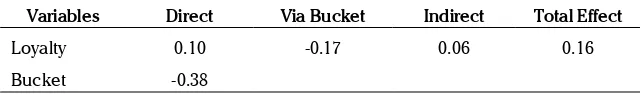
Table 19 summarize the previous 2 tables in term of standardized coefficients for Loyalty and Bucket in its relationship with Profitability. From the table, we can see the direct and indirect effect of Loyalty to profitability. Direct effect shows that loyalty has 0.10 effect to profitability while indirect effect through buckets were 0.16 which is higher that direct effect. The indirect effect numbers can be known by multiplying the standardized coefficient of Loyalty to bucket (-0.17) with bucket to profitability (-0.38). Based on this calculation, we will get the indirect effect of loyalty to profitability as equal to 0.06. The total effect of loyalty to profitability is the sum of direct and indiret effect from loyalty to profitability. The total of Direct effect (0.10) and indirect effect (0.06) will be equal to 0.16.
Figure 5 shows the overall result of this research. The numbers above the arrow shows the standardized coefficient from Dependent Variable into Independent Variable. The R2 shows the regression value of the model. The figure explain the effect of loyalty to buckets and profitability with its strong association numbers.
MANAGERIAL IMPLICATIONS
This paper has proved that loyalty has a significant effect to profitability by way of path analysis. The significane result however, still need to be further elaborated to find a much better tools and additional conclusion. At this point, some implications to marketing startegy that might be proposed is as follow:
• Give more incentive to the customer who stays with the bank for some period of time such as 12 months, 24 months, and 36 months.
Incentive can be given in many ways such as: point rewards, discount on installment payment, small token and others. The main thing is to make customer happy and aware that we know that they have been with us for quite sometimes and we would like to thank them for using our products.
• The same approach can also be done for the customers who were able to achieve a specific period of tenure such as 50%, 80%, etceteras, and a point where actually the bank had received back its principle loan which was disbursed to the customers. Congratulate them for such achievements while keep on motivating them to finish the loan with the bank.
• Cross sell is another way to bind the customer with the bank. Let the customer feel the overall service from the bank, not only from consumer credit products but also other products such as insurance, deposits and investment. One roof solution will make the customer happy and beneficial for the bank.
Active loyalty is above everything. Bank will receive direct and indirect benefit from those customers who recommend its products to his friends, family and relatives. This behavior needs to get extra attention because this is the true value of loyalty, customer feel happy and therefore they offer the same product to the other. Bank did not have to pay for their salary, did not have to pay advertisement, did not have to provide working space for the customers, but yet, application comes in because its customer help them to do it. This customer has to be maintained and awarded equal to their contribution to the bank.
CONCLUSION
There were few findings can be found in this research. Through hypothesis testing, the findings are as follow:
• It was confirmed that loyalty altogether with buckets has a significant effect to profitability. The regression and ANOVA result prove the hypothesis
• It was confirmed that loyalty has a significant effect to buckets, however to have a better sensitivity, it will still need further methodology modification and therefore can show a much better precision.
• The direct and indirect effect of loyalty can be calculated and it shows that loyalty has a positif effect to profitability. The finding confirm many previous research which resulted in the same conclusion using various of different methodology.
• Buckets as representive of days past due, shows a significant effect to profitability. However, as loyalty also has a significant effect to buckets, it can be assumed that loyalty still have its effect even when days past due had reached late stage bucket.
R E F E R E N C E S
Backman SJ, Crompton JL. (1991). Differentiating between high, spurious, latent, and low loyalty participants in two leisure activities. Journal of Park andRecreation Administration 9(2): 1-17.
Baloglu S. (2002). Dimensions of customer loyalty: Separating friends from well-wishers. Cornell Hotel and Restaurant Administration Quarterly 43 (1): 47 – 59.
Baumann C, Burton S, Elliott G. (2007). Predicting Consumer Behavior in Retail Banking. Journal of Business and Management 13(1): 79-96.
Cheng CH, Chen YS. (2009). Classifying the segmentation of customer value via RFM model and RS theory, Expert system with applications, International Journal 3: 4176 – 4184.
De Ruyter K, Bloemer J. (1998). Customer loyalty in extended service settings: The interaction between satisfaction, value attainment and positive mood. International Journal of Service Industry Management 10(3): 320-36.
Dick A, Basu K. (1994). Customer loyalty: toward an integrated framework. Journal of the Academy of Marketing Science 22 (2): 99 – 113.
Eakuru N, Mat N. (2008). The Application of Structural Equation Modeling (SEM) in Determining the Antecedents of Customer Loyalty in Banks in South Thailand. The Business Review Cambridge 10(2): 129-139.
Finlay S. (2008). The Management of Consumer Credit: Theory and Practice. Palgrave Macmillian. New York. Ford J. (1990). Credit and Default Amongst Young Adults: An Agenda of Issues. Journal of Consumer Policy 13(2): 133. Hallowell R. (1996). The relationships of customer satisfaction, customer loyalty, and profitability: an empirical
study. International Journal of Service Industry Management 7(4): 27-42
Hepworth M, Mateus P. (1994). Connecting customer loyalty to the bottom line, Canadian Business Review 21 (4): 40-4. Hoe, S. L. (2008). Issues and Procedures in Adopting Structural Equation Modeling Technique, Journal of Applied Quantitative
Methods, Vol. 3, No. 1, pp. 76-83
Hoelter, D. R.(1983). The analysis of covariance structures: Goodness-of-fit indices, Sociological Methods and Research, Vol. 11, pp. 325–344.
Hughes AM. (1994). Strategic database marketing. Chicago. Probus Publishing Company. Jacoby J, Chestnut R. (1978). Brand Loyalty Measurement and Management. New York. Wiley. Jones TO, Sasser WE. (1995). Why Satisfied Customers Defect, Harvard Business Review 73: 88-99.
Kaymak U. (2001). Fuzzy target selection using RFM variables. IFSA World congress and 20th NAFIPS international conference
2: 1038– 1043.
Kotler P. (1994). Marketing management: Analysis, planning, implementation, and control. New Jersey. Prentice-Hall. Kumar V, Smart PA, Maddern H, Maull RS. (2008). Alternative Perspectives on Service Quality and Customer Satisfaction: The
Lawver M. (1993). Development of a methodology for determining the adequacy of the allowance for loan and lease losses.
Journal of Performance Management 6(1): 50-50.
Lyons AC. (2001). Household liquidity and financial innovations: Evidence from the Survey of Consumer Finances. Ph.D. Dissertation. The University of Texas at Austin, United States - Texas.
Newell F. (1997). The new rules of marketing: How to use one-to-one relationship marketing to be the leader in your industry. New York. McGraw-Hills Companies Inc.
Oliver RL. (1997). Loyalty and profit : long – term effects of satisfaction, satisfaction : A behavioural perspective on the Consumer. New York. MC Graw – Hill Companies Inc.
Oppermann M. (2000). Tourism Destination Loyalty, Journal of Travel Research 39(1): 78 – 84.
Parasuraman A, Zeithaml VA, Berry LL. (1994). Moving forward in service quality research: Measuring different customer-expectation levels, comparing alternative scales, and examining the performance-behavioral intentions link. Working Paper: 94-114, Marketing Science Institute.
Peppers D, Rogers M. (1996). The one to one future: Building relationships one customer at a time New York. Doubleday. Pritchard M, Howard DR. (1997). ,The loyal traveler: Examining a typology of service patronage. Journal of Travel Research
35 (4): 2 – 10.
Reicheld, F.F., Markey, R. G. J., and Hopton C. (2000). The Loyalty effect – the relationship between loyalty and profits,
European Business Journal, 12 (3), 134 - 9
Schijns JMC, Schroder GJ. (1996). Segment selection by relationship strength. Journal of Direct Marketing 10: 69–79.
Selin SW, Howard DR, Udd E, Cable TT. (1987). An analysis of customer loyalty to municipal recreation programs. Leisure Sciences 10: 217 – 23.
Smith L, Jin B. (2007). Modelling exposures to losses on automobile losses. Review of Quantitative Finance & Accounting 29 (3): 241 – 266.
Taylor TB. (1998). Better Loyalty Measurement Leads to Business Solutions. Marketing News, 32 (22): 41-42. Ullman JB. (1996). Structural Equation Modelling. New York. Harper and Row.
Wu J, Lin Z. (2005). Research on customer segmentation model by clustering, ACM International Series :113. Yang K, Trewn J. (2004). Multivariate Statistical Methods in Quality Management. New York. .McGraw-Hill Education. Yoon Y, Uysal M. (2003). An examination of the effects of motivation and satisfaction on destination loyalty: A structural model.