CONTEXT MODELS FOR CRF-BASED CLASSIFICATION OF MULTITEMPORAL
REMOTE SENSING DATA
T. Hoberg*, F. Rottensteiner, C. Heipke
IPI, Institute of Photogrammetry and GeoInformation, Leibniz Universitaet Hannover, Germany (hoberg, rottensteiner, heipke)@ipi.uni-hannover.de
Commission VII, WG VII/4
KEY WORDS: Contextual, Multiresolution, Multitemporal, Land Cover, Classification, Conditional Random Fields
ABSTRACT:
The increasing availability of multitemporal satellite remote sensing data offers new potential for land cover analysis. By combining data acquired at different epochs it is possible both to improve the classification accuracy and to analyse land cover changes at a high frequency. A simultaneous classification of images from different epochs that is also capable of detecting changes is achieved by a new classification technique based on Conditional Random Fields (CRF). CRF provide a probabilistic classification framework including local spatial and temporal context. Although context is known to improve image analysis results, so far only little research was carried out on how to model it. Taking into account context is the main benefit of CRF in comparison to many other classification methods. Context can be already considered by the choice of features and in the design of the interaction potentials that model the dependencies of interacting sites in the CRF. In this paper, these aspects are more thoroughly investigated. The impact of the applied features on the classification result as well as different models for the spatial interaction potentials are evaluated and compared to the purely label-based Markov Random Field model.
* Corresponding author.
1. INTRODUCTION
An increasing number of optical high resolution (HR) remote sensing satellite systems have become available in the last decade. It should thus be possible to improve the classification accuracy and to analyse land cover changes more frequently than this is currently done based on a multitemporal analysis. However, the purchase of HR multitemporal data for these purposes is often not economically viable, especially for large areas. Data having medium resolution do not offer as much detail, but cover a larger area and may often be preferable from an economical point of view. Combining the advantages of both data types requires multiscale and multitemporal analysis.
Up to now most approaches for multitemporal land cover analysis do not make use of temporal dependencies, but derive results by some kind of difference measure between the monotemporal classification results of different epochs (i.e., different acquisition times) (Lu et al., 2004). If data from all epochs are available, it would seem to be advantageous to use the original observations, i.e. the image data, rather than derived data. This has for instance been done in (Feitosa et al., 2009), where a model of temporal dependencies based on Markov chains is applied. As in most techniques for multitemporal classification, each pixel is classified individually without considering spatial context, which leads to a salt-and-pepper-like appearance of the change detection results. Bruzzone et al. (2004) try to overcome this problem by using a cascade of three multitemporal classifiers, one of them considering the k-nearest neighbours of each pixel. A statistical model of spatial context in image classification is given by Markov Random Fields (MRF) (Geman & Geman, 1984), which have also been used for change detection (Melgani & Serpico, 2003), (Moser et al., 2009). In (Melgani & Serpico, 2003), the MRF framework is
extended by a temporal energy term based on a transition probability matrix in order to improve the classification results for two consecutive images. Moser et al. (2009) applied the MRF framework to detect changes in optical satellite images based on multiscale features, but without determining the changed object classes.
Using MRF, the interaction between neighbouring image sites (pixels or segments) is restricted to the class labels, whereas the features extracted from different sites are assumed to be conditionally independent. This restriction is overcome by Conditional Random Fields (CRF; Kumar & Hebert, 2006). CRF provide a discriminative framework that can also model dependencies between features from different image sites and interactions between the labels and the features. In remote sensing CRF have been used for monotemporal classification, e.g. of settlement areas in HR optical satellite images (Zhong & Wang, 2007) or crop types and other land cover classes in Landsat data (Roscher et al., 2010). Multitemporal classification based on CRF for improving the overall classification accuracy as well as detecting changes has first been applied in (Hoberg et al., 2010). This method allows for temporal information passing using an extension of the CRF model.
Multiscale analysis is motivated by the fact that the appearance of objects in a scene is a function of the image resolution and because it is capable of providing a more global view on image content and image analysis algorithms (Kato et al., 1993), (Wilsky, 2002). The simplest way of considering multiple scales in classification is to derive the features at multiple scales, e.g. (Kumar & Hebert, 2006), which has been applied for change detection in (Moser et al., 2009). There have also been approaches to combine a multiscale analysis with CRF. In (Schnitzspan et al., 2008), a multiscale CRF is built on an ISPRS Annals of the Photogrammetry, Remote Sensing and Spatial Information Sciences, Volume I-7, 2012
pyramid structure. Different classes are represented at different scale levels by a part-based object model: at finer resolutions, the classes to be discerned correspond to object parts, whereas at coarser resolutions, they correspond to compound objects. In (Yang et al., 2010) this method is extended to an irregular pyramid based on a multi-scale watershed segmentation of the original image.A combination of multitemporal and multiscale analysis of remote sensing data using CRF is presented by Hoberg et al. (2011). A set of multispectral images of different resolution is classified simultaneously in order to increase the accuracy and reliability of the classification results and to detect land cover changes between the individual epochs. This approach allows to model dependencies between image regions at identical positions in the different epochs that may additionally be characterized by different scales and, hence, by different (though related) class structures.
Unfortunately in publications about CRF there is only little information about feature selection and the influence of different features on the classification result. Moreover in most cases only one model for the interaction potential is applied, without justification of the choice of the particular model. These issues are investigated in this paper. We compare different context models with different subsets of features that are extracted at different scales. First, to find the best subset of features depending on the maximum scale we apply a feature selection process. Next the best feature subset is selected for the association potential. Based on the selected association potential, we investigate three different context models for the spatial interaction potential, again comparing different feature subsets. Finally the results of these investigations are applied in a multitemporal CRF-based classification approach. Tests are performed using two set-ups, one of them using images having identical resolution and one with images of different resolution.
The remainder of this paper is structured as follows. In Section 2, the principles of CRF and the extensions for the classification of multitemporal and multiscale data are presented. Section 3 focuses on the description of the features and on feature selection. In Section 4, the test site is described. A qualitative analysis of the different ways of modelling context is given in Section 5, followed by quantitative results in Section 6. Conclusions and an outlook are given in Section 7.
2. MULTITEMPORAL AND MULTISCALE CRF
In many classification algorithms the decision for a class at a certain image site is just based on information derived at the regarded site (i.e., a pixel, a square block of pixels in a regular grid, or a segment). In fact, the class labels and also the data of spatially and temporally neighbouring sites are often similar or show characteristic patterns, which can be modelled using CRF. In monotemporal classification, we want to determine the vector of class labels x whose components xi correspond to the classes of image sites iS and S being the set of all sites for given called the partition function. The association potentialAi links the class label xi of image site i to the data y, whereas the term addition to the interactions of spatial neighbours, the temporal neighbourhood is taken into account. Each node is only linked to its direct temporal neighbours at its spatial position (Figure 1). The components of the image data vector y are site-wise data vectors yi
t
, with iS and S being the set of sites of all images (i.e., i does not refer to a particular spatial position, but it refers to one spatial position in one of the images). The index t each image site we want to determine the class xi
t
from a set of pre-defined classes. The class structure and thus the number of classes are dependent on t. In order to model the mutual dependency of the class labels at an image site at different epochs, the model for P(x | y) in (1) has to be extended:
(2)
As the different functional models for the potential functions A,
IS, and ITtk are shift-invariant, the subscripts of the potential functions in (1) have been omitted in (2). In (2), A is the association potential, IS the spatial interaction potential that corresponds to the interaction potential Iij in (1), and ITtk the
temporalinteraction potential. In ITtk, yt and yk are the images observed at epochs t and k, respectively. Etis the set of epochs in the temporal neighbourhood of the epoch to which image site
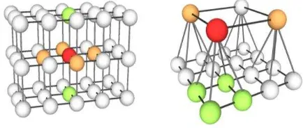
i belongs, thus k is the time index of an epoch in temporal consecutive epochs. The image sites are chosen to be individual pixels and thus are arranged in a regular grid for each image. Figure 1 shows the spatial and temporal neighbourhood for images having identical or different resolutions.
Figure 1. Multitemporal graph structure. Left: images having the same resolution. Right: images having different resolutions. Red nodes: processed primitives; orange / green nodes: spatial / temporal neighbours.
2.1 Association potential
The association potential A(xit, yt) in (2) is related to the probability of label xit taking a value c given the image yt at epoch t by A(xit, yt) = log{P[xit =c | fit(yt)]}. The image data are represented by site-wise feature vectors fit(yt) that may depend on the entire image at epoch t, e.g. by using features at different scales (Kumar & Hebert, 2006). We use a multivariate Gaussian model for P[xit =c | fit(yt)] (Bishop, 2006): features of class c, respectively. It is important to note that both the definition of the features and the dimension of the feature vectors fit(yt) may vary from image to image, because the definition of appropriate and expressive features depends on the image resolution and also on the spectral information contained in the images (see also Section 3).
2.2 Spatial interaction potential
The spatial interaction potential IS(xit, xjt, yt) in (2) is a measure for the influence of the data ytand the neighbouring labels xjton the class xit of image site i at epoch t. In this potential, the data are represented by site-wise vectors of interaction features
ij t
(yt). In this work we compare three different models for the spatial interaction potential. The first model only depends on the labels. It is commonly used with MRF and has a smoothing effect on the labels:
The second model is based on (Shotton et al., 2007):
component-wise differences of the feature vectors hi
t association potential (Kumar & Hebert, 2006). Denoting the mth
component of hit(yt) by himt(yt), the mth component of ijt(yt) is
µijmt = |himt(yt) –hjmt(yt)|. Division by the number of features R in (5) and (6) guarantees an identical influence of the spatial interaction potentials for all images. In IS2 a potential of zero is assigned in the case of two sites have different labels. Differing labels at neighbouring sites are penalized unless the features of the sites are also very different. IS3 penalizes both local changes of the class labels if the data are similar and also identical class labels if the features are different.
2.3 Temporal interaction potential
The temporal interaction potential ITtk(xit, xlk, yt, yk) models the dependencies between the data y and the labels xi
t labels unless it is indicated by differences in the data. However, a more sophisticated functional model would be required to compensate for atmospheric effects and varying illumination conditions, different resolutions, and seasonal effects of the vegetation. We use a simple model for the temporal interaction potential that neglects the dependency of ITtk of the data:
matrix similar to the transition probability matrix in (Bruzzone et al., 2004). The elements of TMs(t)s(k)(xit, xlk) can be seen as conditional probabilities P(xit=ct | xlk=ck) of an image site i belonging to class ct at epoch t if the image site l that occupies the same spatial position as i in epoch k belongs to class ck in that epoch. Qik is the number of elements in Lik and acts as a normalization factor ensuring an identical influence of the sum of all temporal interaction potentials in any epoch, no matter how many temporal neighbours exist. The scales s(t) and s(k) of the data at epochs t and k may differ; there is one matrix
TMs(t)s(k) for each combination of scales available in the data. For further information we refer to (Hoberg et al., 2011).
2.4 Training and Inference
Exact training and inference is computationally intractable for CRF (Kumar & Hebert, 2006). In our application, we only train the parameters of the association potentials, i.e. the mean Efct and the co-variance matrix fc
t
of the features of each class c. They are determined from the features fit(yt) in training sites individually for each epoch t and each class c. The other model parameters, i.e. the weighting factors and of the spatial and temporal interaction potentials and the elements of the transition matrices TMs(t)s(k), were found empirically. For inference, we use Loopy Belief Propagation (LBP) (Nocedal & Wright, 2006), a standard technique for probability propagation in graphs with cycles that has shown to give good results in the comparison reported in (Vishwanathan et al., 2006).
3. FEATURES AND FEATURE SELECTION
In order to apply the CRF framework, the site-wise feature vectors fit(yt) for the association and hit(yt) for the spatial interaction potentials for each epoch t must be defined. Both must consist of appropriate features that can help to discriminate the individual classes. In our application, we used several groups of features, namely colour-based, textural and ISPRS Annals of the Photogrammetry, Remote Sensing and Spatial Information Sciences, Volume I-7, 2012
structural features. All features are computed at five different scales d, with d indicating the scale. Whereas in 1 only individual pixels are taken into account, in 2 to 5 the features are extracted in a square window of size 3, 5, 9, and 13 pixels, respectively, centred at the centre of image site i. Hence we do not only consider information derived at site i for the site-wise feature vectors fi(y) and hi(y), but we also model dependencies between the image information of neighbouring sites.
The colour-based features are directly derived from the pixel defined by Haralick et al. (1973). They are all derived from the gray-level co-occurence matrix that represents the distribution of co-occurring values at a given offset (1 in our case).
The structural features are derived from a weighted histogram of oriented gradients (HOG) (Dalal & Triggs, 2005). Each histogram has 30 bins, so that each bin corresponds to an orientation interval of 6° width. Each bin contains the sum of the magnitudes of all gradients having an orientation that is within the interval corresponding to the bin. Summing over the magnitudes and not just counting the numbers of gradients falling into each bin is done to take into account the impact of strong magnitudes. From the histogram we derive five features: The mean of all gradient magnitudes (Edgrad) the variance of the histogram entries (Vdgrad), the number of bins with magnitudes above the mean magnitude (numd
), the value of the maximum histogram entry (magd) and the angle between the first two maxima (angd). All the features are normalised so that the values are in the interval [0, 1].
We define the feature vectors corresponding to a maximum scale λmax to consist not only of the features extracted at λmax, but also of all features of lower scales. Hence, for instance the feature vector corresponding to max=5 contains 113 elements, nine of them extracted at 1 and 26 features extracted at each additional scale. Using the large number of features just described makes the classification quite time consuming for two reasons: All the features have to be extracted and all have to be considered for determining the potentials. As many of the features are highly correlated or may only marginally support the classification, we apply a feature selection procedure to find out which features are relevant for our aims and to reduce the number of features accordingly. For that purpose we use the correlation-based feature selection approach by Hall (1999). First, the single feature which best classifies the data set is sections, which were processed separately. Seven sections served as training data, the rest as test sites. Ground truth was obtained by manually labelling the images at pixel level. The classes to be distinguished with Ikonos imagery are residential areas (res), industrial areas (ind), forests (for), and cropland (crp). Because there is no clear distinction of the classes res and
ind in the medium resolution Landsat imagery they are fused to a new class built-up areas (bui) in that resolution.
5. FEATURE AND MODEL SELECTION
In this section the impact of using features at different scales and of different context models on the classification result is investigated. We try to find a suitable subset of features for each maximum scale max and then analyse the results to find the best maximum scale and, thus, the optimal feature subset for the association potential. Then we compare different context models for the spatial interaction potential, using the optimal feature subsets for each maximum scale max.
To investigate how many features should be used for our CRF-classification we applied a standard maximum likelihood (ML) classification in subsets with features derived at an increasing number of scales up to a maximum scale λmax, ordering the features according to the results of the feature selection process described above. The ML-classification was chosen because its model is also used for the association potential. For all values of λmax we found that using the six best features was sufficient. Additional features did not further increase the classification accuracy. Hence each of the feature vectors fi
t
(yt) and hi t
(yt) was reduced to just six features depending on max:
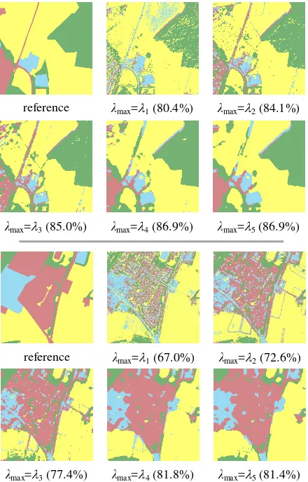
classification obtained for the selected subsets for each value of
max. Figure 2 shows exemplary results for two of the sections using Ikonos imagery; the highest overall accuracy is achieved with max=4. Nevertheless, by visual interpretation most users would consider the result of max=3 to be best, because many finer structures (for instance the road in the upper example of figure 2) are much better preserved. Because information that is lost at this stage cannot be re-introduced in further processing steps, we decided to apply the feature vector fit(yt) for max=3 for the association potential of our further computations. The three context models for the spatial interaction potential (Section 2.2) are evaluated by a monotemporal classification on Ikonos imagery. For the two data-dependent models we used the feature vectors selected for the association potentials in the maximum scales max=
2,
3 and
4 (see above) for hit (yt). In general, the purely label-based model IS1 results in strong smoothing, while the data-dependent models preserve finer structures better, e.g. the road passing through cropland in Figure 3. However, this does not necessarily lead to a higher overall accuracy. In all scales IS2 performs slightly better than IS3, which favours additional class transitions if the features at neighbouring sites are different. The maximum scale of the ISPRS Annals of the Photogrammetry, Remote Sensing and Spatial Information Sciences, Volume I-7, 2012
features in hit(yt) only has a minor effect on the results. Using
max=
2, some salt-and-pepper effects remain, whereas the other scales lead to stronger smoothing. Overall, using IS2 with hit(yt) from max=
3 delivers the best trade-off of overall accuracy and preservation of details assessed by visual impression, which is why this combination is applied in our experiments (cf. Section 6). Hence, in these experiments, fit
(yt) and hi t
(yt) are identical.
6. QUANTITATIVE EVALUTION
We tested our multitemporal approach for two data set-ups: Set-up I has only one scale and consists of two Ikonos images. In the multiscale set-up II we combined one Ikonos and one Landsat scene. For the Ikonos scenes we used the features as defined in Section 5, for the Landsat scene they were extracted only in the original resolution.
The temporal transition matrix TM between Ikonos and Landsat used in our experiments is shown in Table 1. A similar matrix was defined for the transition between the two HR images in set-up I. The choice of these values is dependent on the land cover structure and the assumed changes. We assume that it is most likely to have no changes in any region. Nevertheless each class transition might happen, but with different probability.
xit+1=bui xit+1=for xit+1=crp
xit=res 1 0.05 0.05
xit=ind 1 0.05 0.05
xit=for 0.2 1 0.1
xi t
=crp 0.2 0.1 1
Table 1: Temporal transition matrix; t corresponds to the Ikonos image, t+1 corresponds to the Landsat image. For both set-ups, we compared our method (scenario CRFmulti) to a Maximum Likelihood classification using the Gaussian model in (3) (scenario ML) and to a multitemporal MRF-classification (scenario MRF) using the same graph structure as for our CRFmulti approach, but applying IS1. For these three scenarios, the overall classification accuracy and the kappa coefficients are compared for all epochs in Table 2. In both set-ups we achieved an overall accuracy of over 80% for all images with CRF and MRF, which is an increase of about 8% compared to the monotemporal ML-classification for the Ikonos images and even 15% for the Landsat scene (Figure 4). The impact of the multi-temporal approach is highlighted by the overall accuracy achieved in the scenario CRFmulti in comparison with the results of a monotemporal CRF classification (CRFmono) for the Landsat scene. Using CRFmono only leads to an accuracy of 72%, which is 12% lower than with
CRFmulti. The higher information content of the HR images clearly propagates to the medium resolution scene and yields a significant increase. Nevertheless the accuracy of the HR image also increases. There was hardly any difference between scenarios MRF and CRFmulti. Only in a few regions finer structures are better preserved by the CRF-approach.
S/E ML CRFmulti MRF
I /t1 73.7%/0.57 80.8%/0.72 81.3%/0.73 I/t2 72.8%/0.61 81.1%/ 0.72 80.6%/0.72 II /t1 73.7%/0.57 81.8%/0.73 81.9%/0.73 II /t2 69.6%/0.53 84.3%/0.74 84.1%/0.74 Table 2: Overall classification accuracy / kappa coefficients; S/
E: Set-up/epoch; set up I: t1: Ikonos, 2005; t2: Ikonos, 2007; set up II. t1: Ikonos, 2005; t2: Landsat, 2010. reference λmax=1 (80.4%) λmax=2 (84.1%)
λmax=3 (85.0%) λmax=4 (86.9%) λmax=5 (86.9%)
Figure 2. Overall accuracy of ML-classification in dependence on applied maximum scale λmax for feature extraction. Red: res; blue: ind; green: for; yellow: crp.
reference λmax=1 (67.0%) λmax=2 (72.6%)
λmax=3 (77.4%) λmax=4 (81.8%) λmax=5 (81.4%)
IS2, λmax=2 (88.7%) IS3, λmax=2 (88.2%)
IS1 (90.7%)
IS2, λmax=3 (88.6%) IS3, λmax=3 (88.0%)
IS2, λmax=4 (88.4%) IS3, λmax=4 (87.3%) reference
Figure 3. Overall accuracy of CRF-classification with different context models and varying scale λmax for the spatial interaction potential.
7. CONCLUSION
In this work, we evaluated two possibilities for modelling spatial context within a CRF-framework. First the impact of using features extracted at different scales for the association potential was investigated. Neighbourhood dependencies are already taken into account in this step. Large scales result in a severe smoothing, while tiny structures are lost. Furthermore, different context models for the spatial interaction potential were compared. It could be shown that data-dependent models as used for CRF have a better ability to preserve fine structures. The results of these investigations were applied in a CRF-based approach for multitemporal and multiscale image classification. Besides incorporating spatial context, this method uses a model of temporal context by introducing a temporal interaction potential. The overall classification accuracy of all images was improved by at least 8%. The effect of the multitemporal interaction was highlighted in a set-up of an Ikonos and a Landsat image. The overall accuracy of CRFmulti in comparison to CRFmono for the Landsat scene increased at about 12%.
Further research will concentrate on an improvement of the model for the temporal interaction potential, which was kept quite simple in this work. Moreover, tests on different data sets with a focus on the ability of the method for change detection will be carried out.
ACKNOWLEDGEMENT
The research was funded by the German Science Foundation (DFG) under grant HE 1822/22-1. Our CRF-classification is based on the UGM toolbox by Mark Schmidt:
http://people.cs.ubc.ca/~schmidtm/Software/UGM.html.
REFERENCES
Bishop, C. M., 2006. Pattern recognition and machine learning. 1st edition, Springer New York.
Bruzzone, L., Cossu, R., Vernazza, G., 2004. Detection of land-cover transitions by combining multidate classifiers.
Pattern Recognition Letters, 25(13): 1491-1500.
Dalal, N. and Triggs, B., 2005. Histograms of Oriented Gradients for Human Detection. Proc. of IEEE Conference Computer Vision and Pattern Recognition: 886-893.
Feitosa, R. Q., Costa, G. A. O. P., Mota, G. L. A., Pakzad, K., Costa, M. C. O., 2009. Cascade multitemporal classification based on fuzzy Markov chains. ISPRS J. Photogrammetry Remote Sens. 64(2): 159-170.
Geman, G. and Geman, D., 1984. Stochastic relaxation, Gibbs distribution and Bayesian restoration of images. IEEE Trans. on Pattern Analysis and Machine Intelligence, 6(6): 721-741.
Hall, M. A. (1999). Correlation-based Feature Subset Selection for Machine Learning, PhD dissertation, Department of Computer Science, University of Waikato.
Haralick, R.M., Shanmugam, K. und Dinstein, I. (1973). Texture features for image classification. IEEE Transactions on Systems, Man, and Cybernetics, 3(6): 610–622.
Hoberg, T., Rottensteiner, F. and Heipke, C. 2010. Classification of Multitemporal Remote Sensing Data Using Conditional Random Fields. 6th IAPR TC 7 Workshop Pattern
Recognition in Remote Sens.: 4p.
Hoberg, T., Rottensteiner, F. und Heipke, C. (2011). Classification of multitemporal remote sensing data of different resolution using conditional random fields. 1st IEEE/ISPRS Workshop on Computer Vision for Remote Sensing of the Environment, IEEE ICCV Workshops, Barcelona, 235-242. Kato, Z., Berthod, M., Zerubia, J., 1993. Multiscale Markov random field models for parallel image classification. Proc. Fourth Int. Conference on Computer Vision: 253-257.
Kumar, S. and Hebert, M., 2006. Discriminative Random Fields. Int’l. J. Computer Vision, 68(2): 179-201.
Lu, D., Mausel, P., Brondizio, E., Moran, E., 2004. Change detection techniques. Int. J. Remote Sensing, 25(12): 2365-2401.
Melgani, F. and Serpico, S. B., 2003. A Markov Random Field approach to spatio-temporal contextual image classification.
IEEE-TGARS, 41(11): 2478-2487.
Moser, G., Angiati, E., Serpico, S. B., 2009. A contextual multiscale unsupervised method for change detection with multitemporal remote-sensing images. Proc. 9th Conf. Intelligent Systems Design & Applications: 572-577.
Nocedal, J. and Wright, S. J., 2006. Numerical Optimization.
2nd edition, Springer New York.
Roscher, R., Waske, B., Förstner, W., 2010. Kernel discriminative random fields for land cover classification. 6th
IAPR TC 7 Workshop Pattern Recognition in Remote Sens.: 5p. Schnitzspan, P., Fritz, M., Schiele, B., 2008. Hierarchical support vector random fields: joint training to combine local and global features. Proc. ECCV II: 527-540.
Shotton, J., Winn, J., Rother, C., Criminisi, A., 2007. TextonBoost for Image Understanding: Multi-Class Object Recognition and Segmentation by Jointly Modeling Texture, Layout, and Context. International Journal of Computer Vision, 81(1): 2-23.
Vishwanathan, S., Schraudolph, N. N., Schmidt, M. W., Murphy, K. P., 2006. Accelerated training of conditional random fields with stochastic gradient methods. 23rd Int. Conf. on Machine Learning: 969-976.
Wilsky, A. S., 2002. Multiresolution Markov models for signal and image processing. Proc. IEEE, 90(8): 1396-1458.
Yang, M. Y., Förstner, W., Drauschke, M., 2010. Hierarchical conditional random field for multi-class image classification. Proc. Int’l. Conf. Computer Vision Theory and Applications (VISAPP): 464-469.
Zhong, P. and Wang, R., 2007. A multiple conditional random fields ensemble model for urban area detection in remote sensing optical images. IEEE-TGARS, 45(12): 3978-3988. Figure 4. left: Reference of full test scene (Landsat); middle:
Results of ML; right: Results of CRFmulti: yellow: crp; green: for; dark red: bui; white patches: training areas.