Electronic Journal of Qualitative Theory of Differential Equations
Proc. 8th Coll. QTDE, 2008, No. 141-32; http://www.math.u-szeged.hu/ejqtde/
MULTIPLE PERIODIC SOLUTIONS AND
COMPLEX DYNAMICS FOR SECOND ORDER ODES
VIA LINKED TWIST MAPS
ANNA PASCOLETTI, MARINA PIREDDU, FABIO ZANOLIN
Abstract. We consider some nonlinear second order scalar ODEs of the formx′′+f(t, x) = 0,where f is periodic in thet–variable
and show the existence of infinitely many periodic solutions as well as the presence of complex dynamics, even in the case of certain apparently “simple” equations. We employ a topological approach based on the study of linked twist maps (and suitable modifications of their geometry).
2000 AMS subject classification : 34C25, 37C25, 37D45.
keywords and phrases : Nonlinear second order ODEs, periodic solutions, chaotic dynamics, linked twist mappings.
1. Introduction
The principal aim of this paper is that of proving in a rigorous way (and without the need of computer assistance) the existence of infinitely many periodic solutions and the presence of chaotic dynamics for some nonlinear second order scalar ordinary differential equations (from now on ODEs) of the form
x′′+f(t, x) = 0, (1.1) where f is periodic in the t–variable. In particular, we’ll focus our study on some special cases of equation (1.1), like
x′′+g(x) =p(t),
or
x′′+q(t)g(x) = 0,
but we stress that our approach is, in principle, applicable also to more general equations, including examples in which a term depending onx′ is present in (1.1).
THIS PAPER IS IN FINAL FORM AND NO VERSION OF IT IS SUBMITTED FOR PUBLICATION ELSEWHERE.
The tools which are employed are a combination of a careful but ele-mentary phase–plane analysis with recent results on topological horse-shoes and fixed points for maps defined on domains homeomorphic to the unit square ofR2 [33, 34, 35].
Investigating our ODE models [32, 34, 38] we have found that the Poincar´e map associated to various first order planar systems presents some features which are typical of those usually connected with the so–called “linked twist maps”. Thus a second goal of this work is that of providing a general geometrical setting which is particularly suited to deal with such kind of examples.
The plan of the article is the following. In Section 2 we explain the main topological theory, indicating also the precise definition of chaos we use. In Section 3 we introduce the framework of linked twist maps, concentrating in particular on their geometrical configurations and showing the connection with the theory previously exposed. These topological results are then applied to concrete examples in Section 4, where we show how the phase–portraits of some planar ODE systems recall the geometry associated to the linked twist maps. Part of the results collected in this work surveys some recent theorems from [34, 35, 36, 38, 40]; however, they are here presented from a different point of view, including also new applications.
2. Fixed points, periodic points and chaotic–like dynamics for a class of planar maps
W´ojcik [49], Kennedy and Yorke [15, 16, 17] and further developed in subsequent papers (see also [13, 14, 29, 39, 48, 58, 59, 60], just to quote some recent works in this area).
We start with a few definitions.
Let X be a metric space. By a path γ in X we mean a continuous mappingγ :R⊇[a, b]→X.We also set ¯γ :=γ([a, b]).Of course, there
is no loss of generality in assuming, as a basic interval, [a, b] = [0,1].A sub–path σ of γ is the restriction of γ to a compact subinterval of its domain. An arc is the homeomorphic image of the compact interval [0,1], while an open arc is an arc without its end–points. We define a generalized rectangle as a set R ⊆ X which is homeomorphic to the unit square Q := [0,1]2 ⊆ R2. If R is a generalized rectangle and
h : Q → h(Q) = R is a homeomorphism defining R, we call contour
ϑR of R the set
ϑR :=h(∂Q),
where ∂Q is the usual boundary of the unit square. Note that the contour ϑR is well defined and it is independent of the choice of the homeomorphism h. In fact, ϑR is also a homeomorphic image of S1,
that is, a Jordan curve (the image of a simple closed curve). By an oriented rectangle we mean a pair
e
R := (R,R−),
where R ⊆X is a generalized rectangle and
R− :=R−l ∪ R−r
is the union of two disjoint arcs R−l ,R−
r ⊆ ϑR, called the left and
the right components ofR−. Since ϑR is a Jordan curve we have that
ϑR\(R−l ∪R−
r ) consists of two open arcs. We denote byR+the closure
of such open arcs, calledR+d and R+
u (thedown andup components of
R+). It is important to notice that we can always label the arcs R−
l ,
R+
d ,R−r and R+u,following the cyclic order l−d−r−u−l, and take
a homeomorphism h :Q → h(Q) = R so that the left and right sides ( {0} ×[0,1] and {1} ×[0,1] ) of Q are mapped onto R−l and R−
r ,
while the lower and upper sides ( [0,1]× {0}and [0,1]× {1}) of Qare mapped onto R+d and R+
u , respectively (see Figure 1).
Figure 1. Example of an oriented rectangle embedded in the plane. The [·]−–components of the boundary are drawn
with a thick dark line.
and it was also employed (in a more or less explicit form) by various authors in many different contexts [7, 9, 30].
Lemma 2.1. [Crossing Lemma]. Let Re := (R,R−) be an oriented rectangle in a metric space X and suppose that S ⊆ R is a compact set such that
S ∩γ¯6=∅,
for each path γ : [0,1] → R satisfying γ(0) ∈ R−l and γ(1) ∈ R−
r .
Then there exists a compact connected set C ⊆ S such that
C ∩ R+
d 6=∅, C ∩ R
+
u 6=∅.
Proof. We give only a sketch of the proof. The missing details can be found in [45] or in [34, 35].
such that
A∩ [0,1]× {0}6=∅, A∩ [0,1]× {1}=∅, B ∩ [0,1]× {1}6=∅, B∩ [0,1]× {0}=∅.
The contradiction is now achieved by showing that there is a path σ
contained in Q \ S and joining the left and the right sides of Q (see Figure 2). The existence of such a special path avoidingS =A∪B may be proved by different techniques of topological or combinatorial nature (see, for instance [12, 20, 46] and [37] for a more detailed discussion of
[image:5.595.242.373.314.452.2]these and related results).
Figure 2. A pictorial explanation to the proof of Lemma 2.1.
The above Crossing Lemma may be used to give a simple proof of the Poincar´e–Miranda theorem in dimension two. We recall that the Poincar´e–Miranda theorem asserts the existence of a zero for a continu-ous vector fieldF = (F1, F2) defined on a rectangle [a1, b1]×[a2, b2]⊆R2 and such that F1(a1, x2) ≤ 0 ≤ F1(b1, x2), for every x2 ∈ [a2, b2] and
F2(x1, a2) ≤ 0 ≤ F2(x1, b2), for every x1 ∈ [a1, b1]. Actually, different combinations on the signs of F1 and F2 on the sides of the rectangle are allowed: the only crucial condition requires that the components of the vector field change their sign as the corresponding variables move from a side of the rectangle to the opposite one. The result holds also for the standard hypercube of RN (as well as for N–dimensional
announced this result with a suggestion of a correct proof using the Kronecker’s index. In [42], with regard to the two–dimensional case, Poincar´e (assuming strict inequalities for the components of the vector field on the boundary of the rectangle) described also an heuristic proof as follows: the “curve”F2 = 0 departs from a point of the side x1 =b1 and ends at some point of x1 = a1; in the same manner, the curve
F1 = 0,departing from a point of x2 =b2 and ending at some point of
x2 =a2, must necessarily meet the first “curve” in the interior of the rectangle. The interested reader may find in [19, 23] more information and historical remarks about the Poincar´e–Miranda theorem.
Using Poincar´e’s heuristic argument, one could adapt his proof in the following manner: if we take any path γ(t) contained in the rectangle [a1, b1]×[a2, b2] and joining the left and the right sides, by the Bolzano theorem we find at least a zero ofF1(γ(t)) and this, in turns, means that any path as above meets the set S := F1−1(0). The Crossing Lemma implies the existence of a compact connected set C1 ⊆ F1−1(0) which intersects the lower and the upper sides of the rectangle. At this point one can easily achieve the conclusion in various different ways. For instance, one could just repeat the same argument on F2 in order to obtain a compact connected set C2 ⊆ F2−1(0) which intersects the left and the right sides of the rectangle and thus prove the existence of a zero of the vector fieldF using the fact that C1∩ C2 6=∅.Alternatively, one could apply the Bolzano theorem and find a zero forF2 restricted to C1 (see also [45] for a similar use of a variant of the Crossing Lemma and [40] for extensions to theN–dimensional setting). It may be interesting to observe that, conversely, it is possible to provide a proof of the Crossing Lemma via the Poincar´e–Miranda theorem (see [35]).
Suppose that φ : X ⊇ Dφ → X is a map defined on a set Dφ and
let Ae:= (A,A−) and Be:= (B,B−) be oriented rectangles in a metric spaceX.Now we introduce the concept of “stretching along the paths” which plays a central role in our approach.
Definition 2.1. LetH ⊆ A∩Dφbe a compact set. We say that (H, φ)
stretches Aeto Bealong the paths and write
(H, φ) :Ae−→≎ Be,
if the following conditions hold:
• for every path γ : [a, b] → A such that γ(a) ∈ A−
l and γ(b) ∈
A−
r (or γ(a) ∈ A−r and γ(b) ∈ A−l ), there exists a subinterval
[t′, t′′]⊆[a, b] such that
γ(t)∈ H, φ(γ(t))∈ B, ∀t ∈[t′, t′′]
and, moreover,φ(γ(t′)) andφ(γ(t′′)) belong to different compo-nents ofB−.
In the special case in which H =A,we simply write
φ :Ae−→≎ Be.
The definition of “crossing number” considered below is borrowed from Kennedy and Yorke [17] and adapted to our setting.
Definition 2.2. Let D ⊆ A ∩Dφ be a compact set and let m ≥2 be
an integer. We say that (D, φ) stretches Aeto Be along the paths with crossing number m and write
(D, φ) :Ae−→≎mBe,
if there exist m pairwise disjoint compact sets
H1, . . . ,Hm ⊆ D
such that
(Hi, φ) :Ae−→≎ Be, i= 1, . . . , m.
In the special case in which D =A,we simply write
φ :Ae−→≎mBe.
Our first main result in this section concerns the existence and the localization of at least one fixed point for maps with the stretching property.
Theorem 2.1. Let φ : X ⊇ Dφ → X (with X a metric space) be a
map and Re = (R,R−) be an oriented rectangle with R ⊆ X. Suppose that there is a compact set
H ⊆ R ∩Dφ
such that
(H, φ) :Re−→≎ Re.
Then there exists a point w∈ H with φ(w) =w.
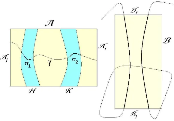
Figure 3. A visual explanation concerning Definition 2.1 and Definition 2.2: the rectanglesAand B,embedded in the plane, have been oriented by selecting, respectively, the sets A− and B− (drawn by thick lines). We have darkened two
compact subsets H and K of A.In the picture, we describe the action of a map φ such that (H, φ) : Ae−→≎ Be and also (K, φ) : Ae−→≎ Be. For a path γ : [0,1] → A with γ(0) and γ(1) belonging to different components of A−, we have put in evidence two restrictions (sub–paths)σ1andσ2with range
in H and K, respectively, such that their composition with φdetermines two new paths (drawn by bolder vertical lines) with values inBand connecting the two different components ofB−.In this case, we could also write φ:Ae−→≎2
e B.
Proof. Like in the proof of Lemma 2.1, it is convenient to reduce our problem to the unit square Q, looking for a fixed point of the map
h−1◦φ◦h.Actually, in order to avoid cumbersome notation, we assume (without loss of generality) R =Q and
(H, φ) :Qe−→≎ Qe,
where we give the natural orientation to Q, setting Qe= (Q,Q−), with Q−
l = {0} ×[0,1] and Q−r = {1} ×[0,1], as well as Q+d = [0,1]× {0}
and Q+
Forφ = (φ1, φ2) and x= (x1, x2), we define the set
S :={x∈ H: 0≤φ2(x)≤1, x1−φ1(x) = 0},
which is compact, as it is closed inQ(this follows from the continuity of
φ on the closed set H). Consider now a path γ = (γ1, γ2) : [0,1]→ Q with γ1(0) = 0 and γ1(1) = 1. By the stretching assumption, there exists an interval [t′, t′′]⊆[0,1] such that
γ(t)∈ H, φ(γ(t))∈ Q, ∀t∈[t′, t′′]
and φ1(γ(t′)) = 0, φ1(γ(t′′)) = 1, or φ1(γ(t′)) = 1, φ1(γ(t′′)) = 0. The continuous function g(t) := γ1(t)−φ1(γ(t)), for t ∈ [t′, t′′], satisfies
g(t′) ≥ 0 ≥ g(t′′), or g(t′) ≤ 0 ≤ g(t′′), respectively, and therefore there exists t∗ ∈[t′, t′′] with γ(t∗)∈ S.Then, by Lemma 2.1, there is a compact connected set C ⊆ S such that C ∩ Q+d 6=∅ and C ∩ Q+
u 6=∅.
By definition of S we know that φ2(w) ∈ [0,1],∀w ∈ C. Hence, for every P = (p1, p2) ∈ C ∩ Q+d we have p2 −φ2(P) ≤ 0 and, similarly, p2 −φ2(P) ≥ 0 for every P = (p1, p2) ∈ C ∩ Q+u . Bolzano theorem
guarantees the existence of at least a pointw= (w1, w2)∈ C such that
w2−φ2(w) = 0. By the inclusion H ⊇ S ⊇ C, we conclude also that
w1−φ1(w) = 0 with w ∈ H and therefore w is a fixed point for φ in
H.
The next step consists in proving the existence of infinitely many periodic points for a given map φ. This is obtained by repeatedly ap-plying Theorem 2.1 to the iterates of φ (see Theorem 2.2). To such end, we first observe that the stretching property is preserved under composition of maps. Indeed, we have:
Lemma 2.2. Let φ :X ⊇Dφ →X and ψ : X ⊇ Dψ →X (with X a
metric space) be such that
(H, φ) :Ae−→≎ Be and (K, ψ) :Be−→≎ Ce,
where Ae, Be, Ceare oriented rectangles in X and
H ⊆ A ∩Dφ and K ⊆ B ∩Dψ
are compact sets. Then
(R, ψ◦φ) :Ae−→≎ Ce, for R :=H ∩φ−1(K).
The proof is a simple adaptation of that in [38, Lemma B.3, Appendix B] (where the caseX =R2 was considered) and therefore it is omitted.
By induction this lemma can be extended to the composition of an arbitrary number of maps.
Theorem 2.2. Let φ : X ⊇ Dφ → X be a map and Re = (R,R−)
an oriented rectangle of the metric space X. Suppose that there are a compact set D ⊆ R ∩Dφ and an integer m≥2 such that
(D, φ) :Re−→≎mRe.
Let also
H1, . . . ,Hm ⊆ D
be m pairwise disjoint compact sets according to Definition 2.2. Then the following conclusions hold:
• for each i = 1, . . . , m, the map φ has at least a fixed point
wi ∈ Hi;
• let ℓ ≥ 2 and consider an arbitrary ℓ+ 1–tuple (s0, s1, . . . , sℓ)
with si ∈ {1, . . . , m}, for all i= 0, . . . , ℓ and such that s0 =sℓ.
Then there exists at least a point w∈ Hs0 such that
φ(ℓ)(w) =w and φ(i)(w)∈ Hsi, ∀i= 1, . . . , ℓ−1.
Proof. The existence of a fixed point for φ in each of the Hi’s follows
from Theorem 2.1 and the fact that
(Hi, φ) :Re−→≎ Re, ∀i= 1, . . . , m.
Consider now the second part of the statement. Let (s0, s1, . . . , sℓ)
be an arbitrary ℓ+ 1-tuple (for ℓ ≥ 2) with si ∈ {1, . . . , m}, for all i = 0, . . . , ℓ and such that s0 = sℓ. Applying Lemma 2.2 to φ(ℓ), we
have that
(W, φ(ℓ)) :Re−→≎ Re,
for the set
W :={x∈ Hs0 : φ
(i)(x)∈ H
si,∀i= 1, . . . , ℓ}
and so Theorem 2.1 ensures the existence of a fixed point w ∈ W for
φ(ℓ). The definition of W implies that w ∈ H
s0 and φ
(i)(w) ∈ H
si, for
The result below gives information about the set of initial points which generate trajectories following an arbitrary forward itinerary. In the sequel, unless otherwise stated, sequences are one–sided and therefore are indexed on the set N of natural numbers. The two–sided
sequences are indexed on Z.
Theorem 2.3. Let φ : X ⊇ Dφ → X be a map and Re = (R,R−)
an oriented rectangle of a metric space X. Suppose that there are a compact set D ⊆ R ∩Dφ and an integer m≥2 such that
(D, φ) :Re−→≎mRe.
Let also
H1, . . . ,Hm ⊆ D
be m pairwise disjoint compact sets according to Definition 2.2. Then the following conclusions hold:
• for each sequence s = (sn)n ∈ {1, . . . , m}N there exists a com-pact connected set Cs⊆ Hs0 satisfying
Cs∩ R+
d 6=∅, Cs∩ R
+
u 6=∅
and such thatφ(i)(x)∈ H
si, ∀i≥1, ∀x∈ Cs; • for each two–sided sequence(sn)n∈Z ∈ {1, . . . , m}
Z
there exists a sequence of points(xn)n∈Zsuch thatφ(xn−1) =xn ∈ Hsn, ∀n∈
Z.
Proof. We start by proving the first assertion. Lets= (sn)n ∈ {1, . . . , m}
N
be an arbitrary sequence and define the set
Ws :={z ∈ Hs0 : φ
(i)(z)∈ H
si, ∀i≥1}.
Let γ0 : [0,1] → R be a path such that γ0(0) and γ0(1) belong to different components ofR−.By the stretching assumption, there exists a subinterval
[t′1, t′′1]⊆[t′0, t′′0] := [0,1] such that
γ0(t)∈ Hs0 and γ1(t) := φ(γ0(t))∈ R, ∀t∈[t
′ 1, t′′1].
By the same assumption, we also have that φ(γ0(t′1)) and φ(γ0(t′′1)) belong to different components of R−. Repeating inductively this ar-gument, we produce a decreasing sequence of compact intervals
[0,1]⊇[t′1, t′′1]⊇[t2′, t′′2]⊇ · · · ⊇[t′n, t′′n]⊇. . .
such that, setting
γn(t) :=φ(γn−1(t)), ∀t∈[t′n, t
′′
n], n≥1,
we have that, for every n ≥0 :
γn(t)∈ R, ∀t∈[t′n, t
′′
n],
γn(t′n), γn(t′′n) belong to different components of R− and
γn(t)∈ Hsn, ∀t∈[t ′
n+1, t′′n+1].
Hence we find that
γ0(t∗)∈ Ws for any t∗ ∈
\
n≥0
[t′n, t′′n].
This proves that any path in R joining the two components of R− meets the set Ws and therefore we can conclude by Lemma 2.1. The second part of the statement (concerning two–sided sequences), follows from a diagonal argument already employed in a more general setting in [14, Proposition 5]. Therefore its proof is omitted (for more
details, see also [34, 36]).
Clearly, Theorem 2.2 and Theorem 2.3 indicate the presence of some kind of chaotic behaviour. To be more precise, we give now the explicit definition of chaos which will be used throughout the paper.
Definition 2.3. Let X be a metric space, let φ :X ⊇ Dφ →X be a
map and D ⊆ Dφ a nonempty set. Let m ≥ 2 be an integer. We say
that φ induces chaotic dynamics on m symbols in the set D if there exist m nonempty pairwise disjoint compact sets
H1,H2, . . . ,Hm ⊆ D
such that, for each two–sided sequence (si)i∈Z ∈ {1, . . . , m} Z
, there exists a corresponding sequence (wi)i∈Z∈ D
Z with
wi ∈ Hsi and wi+1 =φ(wi), ∀i∈Z (2.1)
and, moreover, whenever (si)i∈Z is a k−periodic sequence (that is,
si+k =si,∀i ∈ Z) for somek ≥1, there exists a k−periodic sequence
(wi)i∈Z ∈ D Z
satisfying (2.1). 1
1For k= 1 this simply means that in each of theH
i’s there is at least a fixed
This definition (taken from [18] with minor variants) corresponds to a classical concept of chaos meant as the possibility of reproducing (via the iterates of a map) a general coin–flipping experiment [47, p. 42]. We also note that our definition, when applied to the case of a Poincar´e map, agrees with other ones considered in the literature about chaotic dynamics for ODEs with periodic coefficients (see [8, 31, 49]). We further observe that a connection to the Bernoulli shift can be derived. With this respect, we first recall some basic results.
Letm ≥2 be a positive integer. We denote by
Σm ={1, . . . , m}
Z
the set of the two–sided sequences ofm symbols. The set Σm turns out
to be a compact metric space under a standard metricd.For instance, a possible definition for such a metric is the following:
d(s′,s′′) :=X
i∈Z
|s′i−s′′i| m|i| , s
′ = (s′
i)i∈Z, s′′ = (s′′i)i∈Z ∈Σm.
The Bernoulli shift σ is the homeomorphism on Σm defined by
σ((si)i) := (si+1)i.
As proved in [1], σ has positive topological entropy, given by
htop(σ) = log(m).
Let Λ be a compact metric space and let φ: Λ→Λ be a continuous map. We say that φ issemiconjugate to the two–sided m–shift if there exists a continuous surjective mapping g : Λ→Σm such that
g◦φ =σ◦g. (2.2)
The following lemma relates the dynamical properties of a map satis-fying Definition 2.3 to the ones of the Bernoulli shift.
Lemma 2.3. Let X be a metric space, φ : X ⊇ Dφ → X be a map
which is continuous and injective on a setD ⊆Dφ and induces therein
chaotic dynamics onm≥2symbols (relatively to(H1, . . . ,Hm)). Then,
there exists a nonempty compact set
Λ⊆
m [
j=1 Hj,
with
φ(Λ) = Λ
and such that φ|Λ is semiconjugate to the two–sided m–shift. More-over, the subset P of Λ made by the periodic points of φ is dense in Λ and if we denote by g : Λ→ Σm the continuous surjection in (2.2), it
holds also that the counterimage through g of any k−periodic sequence in Σm contains at least one k−periodic point of φ.
The proof, which is based on arguments presented for instance in [14, 17], is omitted. Complete details can be found in [40]. We observe that the existence of a semiconjugation to the shift map on Σm implies that
the topological entropy ofφ|Λ satisfies
htop(φ|Λ)≥log(m)
(see [53]).
Now we are in position to reconsider Theorem 2.2 and Theorem 2.3 in order to obtain the following:
Theorem 2.4. Let φ : X ⊇ Dφ → X be a map and Re = (R,R−)
an oriented rectangle of a metric space X. Suppose that there are a compact set D ⊆ R ∩Dφ and an integer m≥2 such that
(D, φ) :Re−→≎mRe.
Let also
H1, . . . ,Hm ⊆ D
be m pairwise disjoint compact sets according to Definition 2.2. Then the map φ induces chaotic dynamics on m symbols in the set
H:=
m [
i=1
Hi ⊆ D.
Moreover, for each sequence s = (sn)n ∈ {1, . . . , m}N, there exists a compact connected set Cs⊆ Hs0 with
Cs∩ R
+
d 6=∅, Cs∩ R
+
u 6=∅
and such that, for every w∈ Cs,
In our applications the function φ will the Poincar´e map
φ:z 7→u(T, z)
associated to a T-periodic non–autonomous second order ODE (with
u(·, z) the solution of a given ODE satisfying the initial condition
u(0) =z). In this case, the relation φ(n)(z)∈ Hi will be interpreted in
terms of the oscillatory behaviour of the solutionu(·, z) along the time interval [nT,(n+ 1)T].
3. A connection to linked twist maps
In the past decades a growing interest has concerned the so–called “Linked Twist Maps” (shortly LTMs). Such kind of maps furnish a ge-ometrical setting for the existence of Smale horseshoes and appear in a natural manner in various different applicative contexts. Around the ’80s they were studied from a theoretical point of view by Devaney [10], Burton and Easton [6] and Przytycki [43, 44] (just to cite a few contri-butions in this direction), proving some mathematical properties like ergodicity, hyperbolicity and conjugation to the Bernoulli shift. Spe-cial configurations related to LTMs appear in the restricted three–body problem [28, pp. 90–94], as well as in the study of diffeomorphisms of surfaces or in mathematical models for particle motions in a magnetic field (see the corresponding references in [10]). More recently, in the work of Ottino, Sturman and Wiggins (see, for instance, [50, 54, 55]), LTMs have found applications in the study of fluid mixing. Up to a homeomorphism (or a diffeomorphism), such maps are defined on the union of two circular annuli (or two families of them [44]) intersecting in two different regions. In each annulus a continuous twist mapping is defined, that is, a map which leaves the annulus invariant and rotates its inner and outer boundaries at different angular speeds. Therefore it is possible to consider the composition of the two movements in the common regions: the resulting function is what we call a linked twist map (see [54, 55] for a detailed description of the geometry of the do-main of a LTM). Usual assumptions on the twist mappings involved in the composition require, among others, their smoothness, monotonicity of the angular speed with respect to the radial coordinate and preser-vation of the Lebesgue measure. In our approach (which is purely topological), we’ll just need a twist condition on the boundary.
the linked twist maps. The corresponding theorem (see Theorem 3.1 below) will be then applied to some examples of nonlinear ODEs with periodic coefficients.
Theorem 3.1. Let X be a metric space, let f :X ⊇ Df → X and g : X ⊇Dg →X be continuous maps and letPe:= (P,P−),Oe := (O,O−)
be oriented rectangles in X. Suppose that the following conditions are satisfied:
(Hf) there exist a compact set D ⊆ P ∩Df and an integer m ≥ 2
such that(D, f) :Pe−→≎mOe;
(Hg) O ⊆Dg and g :Oe−→≎ Pe.
Let also H1, . . . ,Hm ⊆ D be m pairwise disjoint compact sets such
that (Hi, f) :Pe−→≎ Oe, for i= 1, . . . , m.
Then the map φ := g◦f induces chaotic dynamics on m symbols in the set H:=∪m
i=1Hi ⊆ D. Moreover, for each sequence of m symbols
s= (sn)n∈ {1, . . . , m}N,there exists a compact connected setCs ⊆ Hs0
with
Cs∩ P
+
d 6=∅, Cs∩ P
+
u 6=∅
and such that, for every w ∈ Cs there exists a sequence (yn)n with y0 =w and
yn∈ Hsn, φ(yn) =yn+1, ∀n≥0.
Proof. We prove
(Hi, φ) :Pe−→≎ Pe, ∀i= 1, . . . , m, (3.1)
from which the conclusion immediately follows by Theorem 2.4. To check condition (3.1), let us consider a path γ : [0,1] → P such that
γ(0) ∈ Pl− and γ(1) ∈ P−
r and let i ∈ {1, . . . , m} be fixed. By (Hf),
there exists a compact interval [t1, t2] ⊆ [0,1] such that γ(t) ∈ Hi
and f(γ(t))∈ O for every t ∈ [t1, t2]. We have also that f(γ(t1)) and
f(γ(t2)) belong to different components ofO−.Just to fix a case for our discussion (the other one is completely analogous), we suppose that
f(γ(t1))∈ Ol−, f(γ(t2))∈ O
−
r .
Define now
σ(t) := f(γ(t)), ∀t∈[t1, t2],
belong to different components ofP−. We have thus showed that
γ(t)∈ Hi and φ(γ(t))∈ P, ∀t ∈[t′, t′′]
with φ(γ(t′)) and φ(γ(t′′)) belonging to different components of P−. This concludes the proof of (3.1) and also of the theorem.
We present now two simple examples for the application of Theorem 3.1 which show how this result is well–fit for studying LTMs. The first of the two examples is fairly classical as it concerns two overlapping annuli under twist rotations. The second one describes the composition of a map which twists an annulus with a longitudinal motion along a strip. Our examples are only of “pedagogical” nature and, in fact, the chaotic–like dynamics that we obtain therein could be also proved using different approaches already developed by various authors (like, for instance, in [27, 48, 56, 60]).
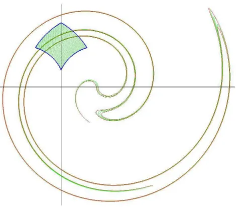
Example 3.1. A classical example of a LTM is represented by the composition of two planar mapsf1 and f2 which act as twist rotations around two given points. For instance, a possible choice is that of considering two maps expressed by means of complex variables as
f1(z) :=−r+ (z+r) exp(ı(e1+a1|z+r|))
and
f2(z) := r+ (z−r) exp(ı(e2+a2|z−r|)),
whereı is the imaginary unit, while r >0, aj 6= 0 and ej (j = 1,2) are
real coefficients. Such maps twist around the centers (−r,0) and (r,0),
respectively. We denote by p1 and p2 the inner and the outer radii for the annulus around (−r,0) and by q1 and q2 the inner and the outer radii for the annulus around (r,0).
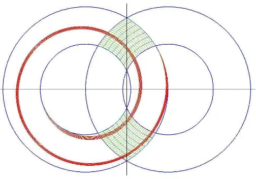
For a suitable choice of r, of the radii p1 < p2 and q1 < q2, as well as of the parameters determining f1 and f2, it is possible to apply Theorem 3.1 in order to obtain chaotic dynamics (see Fig. 4–5).
Figure 4. A pictorial comment to condition (Hf) of The-orem 3.1, with reference to Example 3.1. We have chosen r = 3 and p1 =q1 = 3.3, p2 =q2 = 6 in order to determine
the two annuli (this is just to simplify the example, since no special symmetry is needed). For the mapf1 we have taken
a1 = 3.3 ande1 =−1.5.We define the set P of Theorem 3.1 as the upper intersection of the two annuli and select the two components of P− as the intersections of P with the inner
and outer boundaries of the annulus at the left hand side. The setO is defined as the the lower intersection of the two annuli and the two components of O− are the intersections
of O with the inner and outer boundaries of the annulus at the right hand side. The narrow strip, spiralling inside the left annulus, is the image of P under f1. Clearly, any path
inP joining the two components of P− is transformed byf 1
onto a path crossing Otwice in the correct manner.
this direction, we first introduce, for any pair of real numbers a < b,
the real valued function
P r[a,b](t) := 1
b−a min{b−a,max{0, t−a} },
and then we define
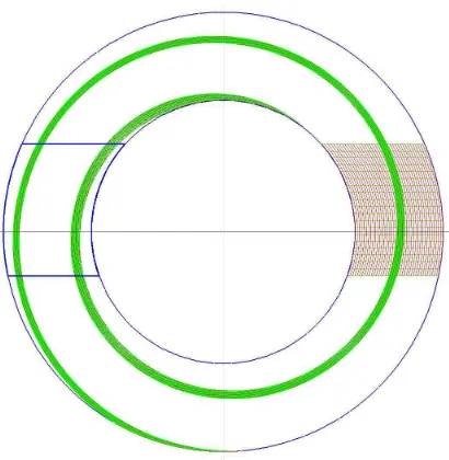
Figure 5. For r, p1, p2, q1, q2 and f1 as in Fig. 4, we have also fixed the parameters off2 by taking a2 = 0.9 and e2 =
0. The present picture shows the image of P through the composite mapf2◦f1.It is evident that (f2◦f1)(P) crosses
P twice in the correct way.
where cj 6= 0 and ej (j = 1,2) are real coefficients and
0< p1 < p2 and −p1 < q1 < q2 < p1
are some real parameters which determine, respectively, the inner and the outer radii of the annulus
A[p1, p2] :={(x, y) : p12 ≤x2+y2 ≤p22}
and the position of the strip
S[q1, q2] := {(x, y) : q1 ≤y≤q2}.
Now we define two maps expressed by means of complex variables as
f1(z) :=zexp(ıg1(|z|))
(which twists around the origin) and, for ℑ(z) = z−z¯ 2ı , f2(z) := z+g2(ℑ(z))
(which shifts the points along the horizontal lines).
possible to apply Theorem 3.1 in order to obtain chaotic dynamics (see Fig. 6–7–8).
Figure 6. A pictorial comment to condition (Hf) of The-orem 3.1, with reference to Example 3.2. We have chosen p1 = 3, p2= 5, q1=−1 andq2= 2 in order to determine the
annulusA[p1, p2] centered at the origin and the stripS[q1, q2]
which goes across it. For the mapf1 we have takene1 = 0.4π
andc1 = 3π.We define the setP of Theorem 3.1 as the right hand side intersection of the annulus with the strip and se-lect the two components ofP− as the intersections ofP with
the inner and outer boundaries of the annulus. The setO is defined as the left hand side intersection of the annulus with the strip and the two components ofO−are the intersections ofOwith the lower and upper sides of the strip. The narrow band, spiralling inside the annulus, is the image of P under f1. Clearly, any path in P joining the two components of
P− is transformed byf
1 onto a path crossing O twice in the
correct manner.
With a straightforward modification in the proof of Theorem 3.1, one could verify that (Hf) and (Hg) imply the existence of chaotic dynamics
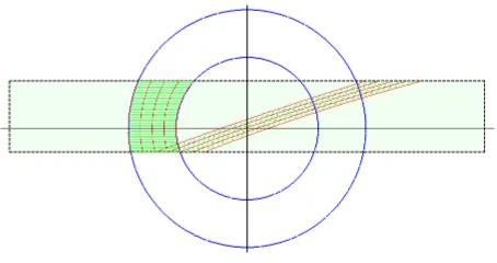
[image:20.595.204.409.190.400.2]Figure 7. A pictorial comment to condition (Hg) of The-orem 3.1, with reference to Example 3.2. We have chosen A[p1, p2] andS[q1, q2] with p1, p2, q1, q2 as in Fig. 6 and
de-fined the oriented rectangles Pe = (P,P−), Oe = (O,O−)
also as before. For the map f2 we have taken e2 = 1 and c2 = 8.6. The parallelogram–shaped narrow figure inside the stripS[q1, q2] is the image of O under f2.Clearly, any path
inO joining the two components ofO− is transformed byf 2
to a path crossing P once in the right way.
Theorem 3.2. Let X be a metric space, letϕ :X ⊇Dϕ →X and ψ : X ⊇Dψ →X be continuous maps and letAe:= (A,A−),Be:= (B,B−)
be oriented rectangles in X. Suppose that the following conditions are satisfied:
(Hϕ) there existm≥1pairwise disjoint compact sets H1, . . . ,Hm ⊆
A ∩Dϕ such that(Hi, ϕ) :Ae−→≎ Be, for i= 1, . . . , m;
(Hψ) there exist ℓ ≥ 1 pairwise disjoint compact sets K1, . . . ,Kℓ ⊆
B ∩Dψ such that (Ki, ψ) :Be−→≎ Ae, for i= 1, . . . , ℓ .
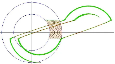
Figure 8. Forp1, p2, q1, q2 and f1 as in Fig. 6 andf2 as in
Fig. 7, we show the image of P through the composite map f2◦f1.It is evident that (f2◦f1)(P) crosses P twice in the
correct manner.
in the set
H∗ := [ i=1,...,m
j=1,...,ℓ H′
i,j with H′i,j :=Hi∩ϕ−1(Kj).
Moreover, for each sequence of m×ℓ symbols
s= (sn)n = (pn, qn)n ∈ {1, . . . , m}N× {1, . . . , ℓ}N,
there exists a compact connected set Cs⊆ H
′
p0,q0 with
Cs∩ A
+
d 6=∅, Cs∩ A
+
u 6=∅
and such that, for every w ∈ Cs, there exists a sequence (yn)n with y0 =w and
Figure 9. In the simple case of Example 3.2 and for f1 andf2determined by the coefficients chosen for drawing Fig.
8, we can determine the sets H1 and H2 in Theorem 3.1.
Indeed, in the setP, transformed in the rectangle [p1, p2]×
[q1, q2] by a suitable change of coordinate, we have found two subsets (drawn with a darker color) whose image through f1 are contained in O. Inside these subsets, we have found
two smaller domains such that their images through f2◦f1
are contained again inP.Clearly, any path contained in the rectangle [p1, p2]×[q1, q2] and joining the left to the right sides contains two sub–paths which are stretched by the composite mapping to paths connecting again the left and the right sides. Up to a homeomorphism between P and [p1, p2]×
[q1, q2],this is precisely what happens in (P,P−) forf2◦f1.
4. An application to second order ODEs
In this section we show a possible application of Theorem 3.1 to the second order scalar ODE
x′′+f(t, x) = 0, (4.1)
where f : R×R → R satisfies the Carath´eodory assumptions and is
T–periodic in the t–variable.
An important subclass of equation (4.1) is given by the periodically perturbed Duffing equations
x′′+g(x) =p(t), (4.2)
whereg :R→R is a locally Lipschitzean function and p(·) :R→Ris
a locally integrable function such thatp(t+T) =p(t),for almost every
t∈R (for some T >0).
as well as of complex dynamics, has been obtained for a special case of equation (4.2). More precisely, in [38] the equation
x′′+kx+ =pr,s(t) (4.3)
has been considered, by assuming that k, r, s, τr, τs are positive real
numbers and pr,s:R→R is a periodic function of period T =Tr,s :=τr+τs,
defined on [0, T[ by
pr,s(t) :=
r , for 0 ≤t < τr,
−s , for τr ≤t < τr +τs,
and then extended to the real line by T−periodicity.
Equation (4.3) can be regarded as a simplified version of the Lazer– McKenna suspension bridges model (see [21, 22]). It is also meaningful from the point of view of the study of ODEs with “jumping nonlin-earities” and the periodic Dancer–Fuˇcik spectrum (see [24] for a very interesting survey concerning recent results in that area).
Our main result is the following:
Theorem 4.1. For any choice of k, r, s > 0 and any positive integer
m ≥ 2, it is possible to find two intervals ]am
r , bmr [ and ]ams , bms [ such
that, for every forcing term pr,s with τr ∈]amr , bmr[ and τs ∈]ams , bms [,
the Poincar´e map associated to (4.3) induces chaotic dynamics on m
symbols in the plane.
In [38, Theorem 1.2], precise information about the oscillatory be-haviour of the solutions is given too. The above result is stable with respect to small perturbations in the sense that once we have proved the existence of chaotic–like dynamics in a certain range of parameters for equation (4.3), then the same result still holds for
x′′+cx′+kx+=p(t) (4.4)
provided that |c| and R0T |p(t)−pr,s(t)|dt (with T =τr+τs) are
suffi-ciently small (see [38, Theorem 1.3] for the details).
We describe now the geometry associated to the phase–portrait of (4.3) in order to show how to apply Theorem 3.1. We remark that similar results can be obtained for equation (4.2) with g a monotone nondecreasing function bounded from below and such that g′(+∞) =
With reference to (4.3), first of all, we observe that the Poincar´e map
φ associated to the equivalent planar system can be decomposed as
φ=φs◦φr,
where φr and φs are the Poincar´e maps
φr :z0 7→ζr(τr, z0), φs :z0 7→ζs(τs, z0)
along the time intervals [0, τr] and [0, τs] associated to the dynamical
systems defined by
(Er)
˙
x=y
˙
y =−kx++r
and
(Es)
˙
x=y
˙
y=−kx+−s.
[image:25.595.170.432.423.524.2]Hereζr(·, z0) denotes the solution (x(·), y(·)) of (Er) with (x(0), y(0)) = z0. Clearly, ζs(·, z0) is defined in the same manner with respect to system (Es).
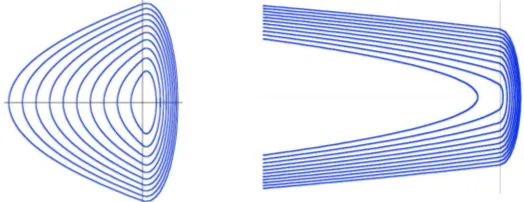
Figure 10. Trajectories of system (Er) (left) and
sys-tem (Es) (right). For this example we have chosen k= 10, r= 4 ands= 0.5.
The orbits of system (Er) correspond to the level lines of the energy
Er(x, y) :=
1 2y
2+ k 2(x
+)2−rx.
Except for the equilibrium point (¯x,0) (with ¯x := r
k), they are closed
On the other hand, the orbits of system (Es) correspond to the level
lines of the energy
Es(x, y) :=
1 2y
2+ k 2(x
+)2+sx.
[image:26.595.186.373.271.523.2]They are run with y′ <0 (see Fig. 10 and Fig. 11).
Figure 11. Example of a trajectory of (Er) (drawn with
a darker line) overlapped with a trajectory of (Es). The
times for moving a point along an orbit from c to ˆx or from ˆx to d can be explicitly determined by means of time–mappings integrals.
Since our trajectories will switch from system (Er) to system (Es)
and viceversa, in order to study the effect of the forcing termpr,s(t),we
are led to overlap the energy level lines of the two systems, as shown in Fig. 11. Next, intersecting two level lines of (Er) with two level lines
Figure 12. Level lines of system (Er) overlapped with
the level lines of system (Es) in the left half plane x≤0.
The setsP andOare those bounded by the four different level lines and contained in the lower half plane y ≤ 0 and in the upper half planey≥ 0, respectively.
In order to get periodic and chaotic solutions for the system
˙
x=y
˙
y =−kx++p
r,s(t) (4.5)
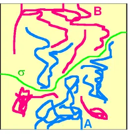
and thus for equation (4.3), we employ the following elementary pro-cedure: we construct a set P in the third quadrant bounded by two level lines of (Er) and two level lines of (Es). Using the fact that the
period T(·) of the closed orbits of system (Er) is a strictly monotone
increasing function on [0,+∞), we define the two components of P− (here denoted by P−
1 andP2− 2) as the intersections of P with the level lines of Er, so that points on the inner boundary move faster than
points of the outer boundary. Hence, if we take a path γ contained in the third quadrant and joining such two boundary segments, we’ll find that (after a sufficiently long time τr) its image through φr turns
out to be a spiral–like line crossing the second quadrant at least twice. In particular, we can select two sub–paths (say σ1 and σ2) of γ whose
2 in order to avoid confusion with the letters r and s already employed in equation (4.3).
images throughφr cross the second quadrant. We also define a
rectan-gular subset O in the second quadrant (which is just the reflection of P with respect to the x–axis) having as components of O− (denoted now by O−1 and O2−) the intersections of O with two level lines of Es
and such that φr(σ1) and φr(σ2) admit sub–paths contained in O and joining O−1 toO−2 . When we switch to system (Es),we can prove that
the images of such sub–paths through φs cross the set P in the right
manner. Then we can apply Theorem 3.1 provided we are free to tune the switching times τr and τs. The technical details for this argument
can be found in [38].
Similar conclusions can be drawn for the second order ODE
x′′+q(t)g(x) = 0, (4.6) withg a nonlinear term andq(·) a periodic step function (or a suitable small perturbation of a step function). In the case of a general (but sign changing) weight function q(t), previous results for this equation have been obtained by Butler [7], Terracini and Verzini [52], Papini and Zanolin [32, 33, 35]. The detection of chaotic–like solutions for (4.6) with a positive q(t) and under general conditions on g(x) appears as an interesting problem which has not yet been fully investigated. Due to space limitations, we confine such study to a future work.
5. Conclusions
In the present article we have shown how to apply the abstract topo-logical theory exposed in Section 2 and already developed in [34, 35] to prove the existence of chaotic dynamics for some concrete equations, whose phase–portrait recalls the geometry of the linked twist maps. Further developments in this direction can be obtained by studying new ODE models, whose Poincar´e map presents features similar, but not corresponding exactly, to that of the classical LTMs. For example, frameworks like the one in Fig. 7 can be considered as well. Suitable variants of such situations will be analyzed in a future paper.
indicate that the same is true also for more general time–dependent coefficients. However, a rigorous proof in such a case would require a more delicate analysis or possibly the aid of computer assistance (as in [3, 4, 26, 27, 57] ). This is far beyond the aims of the present pa-per where, instead, we wanted only to put in evidence the presence of some simple geometric configurations which appear in a natural way in various planar systems and lead to “chaos”.
References
[1] R.L. Adler, A.G. Konheim and M.H. McAndrew, Topological entropy, Trans. Amer. Math. Soc.114(1965), 309–319.
[2] J.C. Alexander, A primer on connectivity,Fixed point theory (Sherbrooke, Que., 1980), Lecture Notes in Math., Springer, Berlin886(1981), 455–483.
[3] B. B´anhelyi, T. Csendes and B.M. Garay, Optimization and the Miranda approach in detecting horseshoe–type chaos by computer, Int. J. Bifurcation and Chaos 17(2007), 735–747.
[4] B. B´anhelyi, T. Csendes, B.M. Garay and L. Hatvani, A computer– assisted proof for Σ3–chaos in the forced damped pendulum equation, (to ap-pear).
[5] K. Burns and H. Weiss, A geometric criterion for positive topological en-tropy,Comm. Math. Phys.172(1995), 95–118.
[6] R. Burton and R.W. Easton, Ergodicity of linked twist maps,Global theory of dynamical systems (Proc. Internat. Conf., Northwestern Univ., Evanston, Ill., 1979), Lecture Notes in Math., Springer, Berlin819(1980), 35–49.
[7] G.J. Butler, Rapid oscillation, nonextendability, and the existence of pe-riodic solutions to second order nonlinear ordinary differential equations, J. Differential Equations 22 (1976), 467–477.
[8] A. Capietto, W. Dambrosio and D. Papini, Superlinear indefinite equa-tions on the real line and chaotic dynamics, J. Differential Equations 181
(2002), 419–438.
[9] C. Conley, An application of Wa˙zewski’s method to a non-linear boundary value problem which arises in population genetics, J. Math. Biol. 2 (1975),
241–249.
[10] R.L. Devaney, Subshifts of finite type in linked twist mappings,Proc. Amer. Math. Soc.71(1978), 334–338.
[11] R.W. Easton, Isolating blocks and symbolic dynamics,J. Differential Equa-tions 17(1975), 96–118.
[12] D. Gale, The game of Hex and the Brouwer fixed-point theorem,Amer. Math. Monthly 86(1979), 818–827.
[13] Z. Galias and P. Zgliczy´nski, Abundance of homoclinic and heteroclinic orbits and rigorous bounds for the topological entropy for the H´enon map, Nonlinearity 14(2001), 909–932.
[14] J. Kennedy, S. Koc¸ak and Y.A. Yorke, A chaos lemma, Amer. Math. Monthly 108(2001), 411–423.
[15] J. Kennedy and J.A. Yorke, The topology of stirred fluids,Topology Appl.
80(1997), 201–238.
[16] J. Kennedy and J.A. Yorke, Dynamical system topology preserved in pres-ence of noise,Tr. J. of Mathematics 22(1998), 379–413.
[17] J. Kennedy and J.A. Yorke, Topological horseshoes,Trans. Amer. Math. Soc.353(2001), 2513–2530.
[18] U. Kirchgraber and D. Stoffer, On the definition of chaos, Z. Angew. Math. Mech.69(1989), 175–185.
[19] W. Kulpa, The Poincar´e-Miranda theorem, Amer. Math. Monthly 104
(1997), 545–550.
[20] W. Kulpa, M. Pordzik, L. Socha and M. Turzanski,L1cheapest paths in “Fjord scenery”,European J. Oper. Res.161(2005), 736–753.
[21] A.C. Lazer and P.J. McKenna, Large scale oscillatory behaviour in loaded asymmetric systems, Ann. Inst. Henry Poincar´e, Analyse non lineaire 4
(1987), 244–274.
[22] A.C. Lazer and P.J. McKenna, Large–amplitude periodic oscillations in suspension bridges: some new connections with nonlinear analysis,SIAM Re-view 32(1990), 537–578.
[23] J. Mawhin, Poincar´e early use ofAnalysis situsin nonlinear differential equa-tions: Variations around the theme of Kronecker’s integral, Philosophia Sci-etiae 4(2000), 103–143.
[24] J. Mawhin, Resonance and nonlinearity: a survey.Preprint 2006.
[25] C. Miranda, Un’osservazione su un teorema di Brouwer,Boll. Un. Mat. Ital. (2)3(1940), 5–7.
[26] K. Mischaikow and M. Mrozek, Chaos in the Lorenz equations: a computer–assisted proof,Bull. Amer. Math. Soc.32(1995), 66–72.
[27] K. Mischaikow and M. Mrozek, Isolating neighborhoods and chaos,Japan J. Indust. Appl. Math.12(1995), 205–236.
[28] J. Moser, Stable and Random Motions in Dynamical Systems. With special emphasis on celestial mechanics, Hermann Weyl Lectures, the Institute for Advanced Study, Princeton, N. J. Annals of Mathematics Studies, No. 77. Princeton University Press, Princeton, N. J., 1973.
[29] M. Mrozek and K. W´ojcik, Discrete version of a geometric method for detecting chaotic dynamics,Topology Appl.152(2005), 70–82.
[30] J.S. Muldowney and D. Willett, An elementary proof of the existence of solutions to second order nonlinear boundary value problems,SIAM J. Math. Anal 5(1974), 701–707.
[31] D. Papini, Prescribing the nodal behaviour of periodic solutions of a super-linear equation with indefinite weight,Atti Sem. Mat. Fis. Univ. Modena 51
(2003), 43–63.
[32] D. Papini and F. Zanolin, A topological approach to superlinear indefinite boundary value problems,Topol. Methods Nonlinear Anal.15(2000), 203–233.
[34] D. Papini and F. Zanolin, On the periodic boundary value problem and chaotic-like dynamics for nonlinear Hill’s equations, Adv. Nonlinear Stud. 4
(2004), 71–91.
[35] D. Papini and F. Zanolin, Fixed points, periodic points, and coin-tossing sequences for mappings defined on two-dimensional cells,Fixed Point Theory Appl.2004(2004), 113–134.
[36] D. Papini and F. Zanolin, Some results on periodic points and chaotic dynamics arising from the study of the nonlinear Hill equations,Rend. Sem. Mat. Univ. Pol. Torino65(2007), 115–157 (Special Issue: Subalpine Rhapsody
in Dynamics).
[37] A. Pascoletti,Punti fissi per mappe del piano con applicazioni alle equazioni differenziali, Tesi di laurea magistrale, University of Udine, 2007.
[38] A. Pascoletti and F. Zanolin, Example of a suspension bridge ODE model exhibiting chaotic dynamics: a topological approach,J. Math. Anal. Appl.339
(2008), 1179–1198.
[39] M. Pireddu and F. Zanolin, Fixed points for dissipative-repulsive systems and topological dynamics of mappings defined on N-dimensional cells, Adv. Nonlinear Stud.5(2005), 411–440.
[40] M. Pireddu and F. Zanolin, Cutting surfaces and applications to periodic points and chaotic–like dynamics,Topol. Methods Nonlinear Anal.(to appear). [41] H. Poincar´e, Sur certaines solutions particuli`eres du probl`eme des trois corps,
C.R. Acad. Sci. Paris 97 (1883), 251–252.
[42] H. Poincar´e, Sur certaines solutions particuli`eres du probl`eme des trois corps, Bulletin Astronomique 91(1884), 65–74.
[43] F. Przytycki, Ergodicity of toral linked twist mappings, Ann. Sci. ´Ecole Norm. Sup. (4)16 (1983), 345–354.
[44] F. Przytycki, Periodic points of linked twist mappings, Studia Math. 83
(1986), 1–18.
[45] C. Rebelo and F. Zanolin, On the existence and multiplicity of branches of nodal solutions for a class of parameter-dependent Sturm-Liouville problems via the shooting map,Differential Integral Equations 13(2000), 1473–1502.
[46] D.E. Sanderson, Advanced plane topology from an elementary standpoint, Math. Mag.53(1980), 81–89.
[47] S. Smale, Finding a horseshoe on the beaches of Rio,Math. Intelligencer 20
(1998), 39–44.
[48] R. Srzednicki, A generalization of the Lefschetz fixed point theorem and detection of chaos,Proc. Amer. Math. Soc.128(2000), 1231–1239.
[49] R. Srzednicki and K. W´ojcik, A geometric method for detecting chaotic dynamics,J. Differential Equations 135(1997), 66–82.
[50] R. Sturman, The linked twist map approach to fluid mix-ing, Dynamical Systems and Statistical Mechanics, London Math-ematical Society Durham Symposium 2006. Available online at: http://www.maths.dur.ac.uk/events/Meetings/LMS/2006/DSSM/talks.html [51] A. Szymczak, The Conley index and symbolic dynamics,Topology 35(1996),
287–299.
[52] S. Terracini and G. Verzini, Oscillating solutions to second- order ODEs with indefinite superlinear nonlinearities,Nonlinearity 13(2000), 1501–1514.
[53] P. Walters, An introduction to ergodic theory, Graduate Texts in Mathe-matics, Vol.79, Springer-Verlag, New York, 1982.
[54] S. Wiggins, Chaos in the dynamics generated by sequence of maps, with application to chaotic advection in flows with aperiodic time dependence, Z. angew. Math. Phys.50(1999), 585–616.
[55] S. Wiggins and J.M. Ottino, Foundations of chaotic mixing,Philos. Trans. R. Soc. Lond. Ser. A Math. Phys. Eng. Sci.362(2004), 937–970.
[56] P. Zgliczy´nski, Fixed point index for iterations of maps, topological horse-shoe and chaos,Topol. Methods Nonlinear Anal.8(1996), 169–177.
[57] P. Zgliczy´nski, Computer assisted proof of chaos in the R¨ossler equations and in the H´enon map,Nonlinearity 10 (1997), 243–252.
[58] P. Zgliczy´nski, Sharkovskii’s theorem for multidimensional perturbations of one-dimensional maps,Ergodic Theory Dynam. Systems19(1999), 1655–1684.
[59] P. Zgliczy´nski, On periodic points for systems of weakly coupled 1-dim maps,Nonlinear Anal. Ser. A: Theory Methods 46(2001), 1039–1062.
[60] P. Zgliczy´nski and M. Gidea, Covering relations for multidimensional dy-namical systems,J. Differential Equations 202(2004), 32–58.
(Received August 30, 2007)
University of Udine,
Department of Mathematics and Computer Science, Via delle Scienze 206, 33100 Udine, Italy
![Figure 1. Example of an oriented rectangle embedded inthe plane. The [·]−–components of the boundary are drawnwith a thick dark line.](https://thumb-ap.123doks.com/thumbv2/123dok/966532.912690/4.595.202.420.136.261/figure-example-oriented-rectangle-embedded-components-boundary-drawnwith.webp)
![Figure 9. In the simple case of Example 3.2 and for f1and f2 determined by the coefficients chosen for drawing Fig.8, we can determine the sets H1 and H2 in Theorem 3.1.Indeed, in the set P, transformed in the rectangle [p1, p2] ×[q1, q2] by a suitable chang](https://thumb-ap.123doks.com/thumbv2/123dok/966532.912690/23.595.184.425.116.233/example-determined-coecients-determine-theorem-transformed-rectangle-suitable.webp)