A New Method for the Explicit
Integration of Lotka-Volterra Equations
Un Nuevo M´
etodo para la Integraci´
on Expl´ıcita
de las Ecuaciones de Lotka-Volterra
Giovanni Mingari Scarpello ([email protected])
via Negroli, 6 20133 Milano Italy
Daniele Ritelli ([email protected])
Dipartimento di Matematica per le Scienze Economiche e Sociali viale Filopanti, 5 40127 Bologna, Italy.
Abstract
In this work we study some first order nonlinear ordinary differential equations describing the time evolution (or “motion”) of those hamilto-nian systems provided with a first integral linking implicitly both vari-ables to a motion constant. An application has been performed on the Lotka-Volterra predator-prey system, turning to a strongly nonlinear differential equation in the phase variables.
Our method grasps all the capabilities of modern computer algebra in order to solve (algebraic approximation) some equations of third and fourth degree with intricate forcing terms, obtaining symbolic explicit expressions osculating the solution in a neighborhood of the initial con-ditions.
Another approach is also developed managing a Taylor truncated series and inverting it (asymptotic approximation). After having eval-uated how both approximations differ from the traditional numerical techniques, finally we accomplish the much more probatory control of the approximants’ accuracy referred, through the motion constant, to the first integral of the equation itself.
Key words and phrases: Lotka-Volterra equations, Lagrange Rever-sion, explicit integration, implicit function theorem.
Recibido 2002/03/13. Revisado 2002/11/06. Aceptado 2003/06/07. MSC (2000): Primary 34A34; Secondary 26B05.
Resumen
En este trabajo se consideran algunas ecuaciones diferenciales de primer orden que describen la evoluci´on temporal (o “movimiento”) de algunos sistemas hamiltonianos dotados de una preintegral que rela-ciona impl´ıcitamente ambas variables a una constante de movimiento. Se realiza una aplicaci´on al sistema predador-presa de Lotka-Volterra, que conduce a una ecuaci´on diferencial fuertemente no lineal en las variables de fase. Nuestro m´etodo aprovecha todas las capacidades de la moderna ´algebra computacional para resolver (aproximaci´on alge-braica) ecuaciones algebraicas de tercer y cuarto grado con t´erminos complicados, obteniendo expresiones simb´olicas expl´ıcitas de funciones que osculan la soluci´on en un entorno de las condiciones iniciales.
Tambi’en se desarrolla otro enfoque basado en la inversi´on una serie de Taylor truncada (aproximaci´on asint´otica). After having evaluated how both approximations differ from the traditional numerical tech-niques, finally we accomplish the much more probatory control of the approximants’ accuracy referred, through the motion constant, to the first integral of the equation itself.
Despu´es de evaluar el modo como nuestras soluciones difieren de aquellas obtenidas con las t´ecnicas num´ericas tradicionales, finalmente se realiza, hecho de mayor evidencia probatoria, un control cuidadoso de la aproximaci´on obtenida referrida, a trav´es de la constante de mo-vimiento, a una preintegral de la misma ecuaci´on.
Palabras y frases clave:Ecuaciones de Lotka-Volterra, reversi´on de Lagrange, integraci´on expl´ıcita, teorema de la funci´on impl´ıcita.
1
Introduction
This paper is devoted to some novel application of the scalar form of the Theorem of implicit functions (see [3] for a historical outline of this theorem) in order to obtain a new treatment for systems of coupled nonlinear ordinary differential equations. Let us recall the theorem’s statement:
Theorem (Ulisse Dini, 1878). Let Ωan open set in R2 and f : Ω→R a C1 function. Suppose there exists(¯x,y¯)∈Ωsuch that:
f(¯x,y¯) = 0, ∂f
∂y(¯x,y¯)>0,
then there must be a real interval B centered around x, a real interval I
• B×I⊂Ω,
• for any(x, y)∈B×I:
∂f
∂y(x, y)6= 0,
• if(x, y)∈B×I then:
f(x, y) = 0,
if and only ify=ϕ(x),
• y¯=ϕ(¯x),
• ϕ∈ C1(B)and for any x∈B:
ϕ′
(x) =−
∂f
∂x(x, ϕ(x)) ∂f
∂y (x, ϕ(x)) .
A careful observation of this theorem’s proof reveals that the most im-portant fact is determining the radius of the intervalB. Indeed if we choose
a, b∈R, a, b >0 such that ifB1= [¯x−a,x¯+a] andI1= [¯y−a,y¯+a] then
Ωa,b=B1×I1⊂Ω,we define:
m= min
Ωa,b
∂f ∂y,
and:
M = 1 + max
Ωa,b
∂f ∂x .
We observe thatm >0, M >0.Therefore the intervalB in the statement of the theorem of implicit functions is any interval of the form:
B= [¯x−δ,x¯+δ] (1.1)
with δ∈]0, a[ and δ≤ mb
2M. This leads to the conclusion that the solution for
y of (1.6) will be defined in the neighborhood (1.1) of (¯x,y¯).
We need the implicit functions theorem for integrating separable nonlinear differential equations. For instance, we could consider the nonlinear problem:
(
˙
y(t) =a(t)b(y(t)), y(t0) =y0,
where a : B → R, b : I → R are real continuous functions on the open
intervals B and I with t0 ∈ B, y0 ∈ I and with b(y0) 6= 0. The unique
solution of the problem is implicitly defined by:
Z y
y0 1
b(ξ)dξ=
Z t
t0
a(η)dη, (1.3)
in such a way the function of two variables:
f(t, y) =
Z y
y0 1
b(ξ)dξ−
Z t
t0
a(η)dη, (1.4)
supplies the implicit solution of (1.2) .
Therefore, we see that the Cauchy problem (1.2) supplies an implicit func-tion problem of the special form:
g(x) =h(y), (1.5)
where g : B → R, h : I → R are two smooth real functions defined in the
open real intervals B, I and where x0 ∈ B, y0 ∈ I and g(x0) = h(y0).
Moreover h′(
y0) 6= 0. The particular form of (1.5) in order to solve for y
the transcendental equation (1.5), suggests the approach of replacing h(y) by its nth order Taylor polynomial evaluated at y0. Of course this requires h ∈ Cn(I), n ∈N, which covers the most occurrences. Thus, if p
n(y, y0) is
thenthorder Taylor polynomial ofh(y) aty
0,instead of (1.5), we will consider
the integration of (1.2) as mapped by solving thenthorder algebraic equation
in y :
g(x) =pn(y, y0). (1.6)
Please note that the degree zero coefficient (the forcing term) of (1.6) depends on the parameterx∈B.We can then state:
Theorem 1. The following facts hold:
1. equation (1.6)meets all the hypotheses of the theorem of implicit func-tions and thus (1.6)will be satisfied by one and only one functionyn=
yn(x, x0);
2. ifhis real analytic, then:
lim
n→∞yn(x, x0) =h
−1(g(x)) =ϕ(x),
whereϕ(x)is the unique function, defined in a suitable subinterval ofB
Proof. The first statement follows immediately becauseh(y) and thenthorder
Taylor polynomialpn(y, y0) have the same derivative at y =y0. The second
property comes down from the following argument. We suppose h(y) real analytic with radius of convergenceρ >0, i.e.:
h(y) =
∞ X
n=0 h(n)(y
0)
n! (y−y0)
n
, |y−y0|< ρ.
It is known (see [2] page 184 chap V. §21 n. 107) that, by means of the Lagrange’s power series reversion theorem, the inverse function, h−1(z) is
analytic too, i.e. his Taylor series converges. Moreover the series’ coefficients are uniquely determined by the Lagrange recursion formula. Of course the same holds for pn(y, y0) thought as a function of y, and if p−n1(z, y0) is the
relevant inverse function, the reversion algorithm ensures that:
lim
n→∞p −1
n (z, y0) =h−1(z).
Finally, we prove thatyn→ϕ(x). In fact:
|yn−y|=
p−1
n (g(x), y0)−h−1(g(x)) →0
as n→ ∞.
Our strategy of finding closed form solutions of (1.2), deals therefore with the classical problem of solving algebraic equations of degree greater than two. In this framework we used Mathematicar with its routines for the symbolic
solution of third and fourth degree equations.1 In the next section we shall
apply our method to the the Lotka-Volterra predator-prey planar system (sans
overcrowding).
2
Algebraic approximations
The Lotka-Volterra predator-prey system of nonlinear differential equations is:
(
˙
u(t) =u(t) −c+dv(t) ,
˙
v(t) =v(t) a−bu(t)
, (2.1)
v(t) andu(t) being the populations of the preys and the predators respectively at the momentt; whilea, b, canddare positive constants of unitst−1, where:
1
• ais the birth rate of the preys,
• bis the proportion of preys actually eaten by the predators,
• cis the rate at which predators die if not nourished,
• dis the biomass conversion constant of the predators.
The main properties of the planar system (2.1) solutions are:
• the first quadrant is an invariant set for all the solutions of (2.1) with positive initial conditions,
• (2.1) has two equilibria: the origin andE= (a
b, c d),
• any solution of (2.1) shall be greater than zero, periodic in the first quadrant and their orbits shall wander around E.
In spite of its simple formulation, no closed form solution of (2.1) is known. However, writing (2.1) as:
d
dt lnu(t)
=−c+dv(t), d
dt lnv(t)
=a−bu(t),
and making the change of variables:
x= lnd
cv
,
y= lnb
au
.
which will moveEto the origin, now the system depends on two parameters
alone, namely aandc:
(
˙
x(t) =a 1−expy(t) ,
˙
y(t) =−c 1−expx(t)
, (2.2)
The initial conditionsx(0) =x0,y(0) =y0 are no longer necessarily positive
and one can immediately obtain the orbit differential equation in the (x, y) plane:
dy dx =k
1−expx
1−expy
,
y(x0) =y0,
k=−c
a <0,
(2.3)
which is of the type (1.2). Therefore due to (1.3), the solution of (2.3) can be found to be:
y−expy=k(x−expx) +C, (2.4)
where:
C=y0−expy0−k(x0−expx0),
is the constant of integration (ormotion constant for people mechanically in-clined), withx0=x(0) andy0=y(x(0)).If (2.4) could be solved explicitly
for y, the orbit of the Lotka-Volterra system would be known: but unfortu-nately the transcendental nonlinearity of (2.4) prevents this. Note that (2.4) is an implicit equation like (1.5): therefore the Dini theorem comes into play. We are going to replace the left hand side of (2.4) with its Taylor expansion: of course this bounds us to work in a neighborhood of the initial value y0 in
order to achieve a reasonably good approximation fory. The solution’s peri-odicity allows us to take the initial data: y(0) =y0 >0 and x(0) =x0 = 0
without loss of generality, the latter being themotion coordinates around the origin of the new logarithmic system.
2.1
Numerical reference solutions of Lotka-Volterra
equations
In order to test the accuracy of the approximate explicit solution we are going to compute, and compare it with the numerical ones, we consider a sample case by fixing the coefficients aand c and the initial valuesx0 andy0. This does
not affect the generality of our method, because the procedure can be easily implemented in different situations; moreover we can so test our accuracy. Let us display the Mathematicar solution first. Let a = 2, c = 1, x0 = 0
etimes their equilibrium value). Then (2.2) and (2.4) can be written as
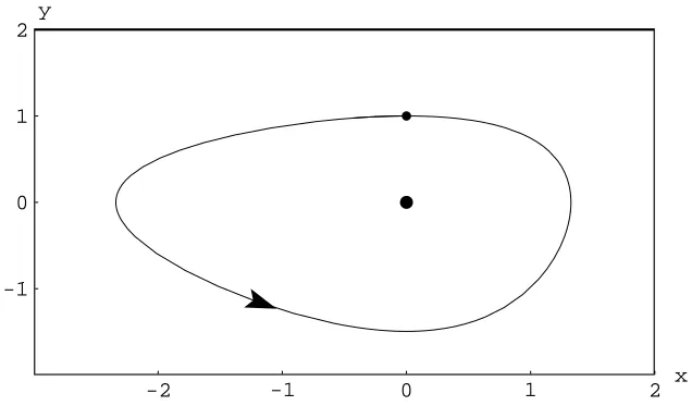
Making use of the packageVisualDSolve.m, by D. Schwalbe and S. Wagon [4], the system’s orbit on the (x, y) plane will be found, and we will be able to store the numerical solution for a later comparison. The orbit 2, which runs counterclockwise, is shown at Figure 3.
Moreover, as suggested in [1], the numerical computation’s accuracy can be checked by the conservation law (2.6). First of all, let us observe that the period of system (2.5) can be numerically computed as τ ≃5.27. Therefore let us introduce the finite subset of the intervalI= [0,5.27]:
Thus making the time span discrete, each time interval will be 500001 of the overall intervalI. Let (x(t), y(t)) denote the solution found by Mathematicar.
Eeplacing the left hand side of (2.6), one finds that
sup
instead of zero. The time span has been also divided into 10000 steps find-ing the error substantially unchanged. This means that Mathematicar’s
predictor-corrector technique provides solutions which differ from themotion
constant by less than 10−4, and therefore are surely correct to four decimal
digits.
2
-2 -1 0 1 2 x -1
0 1 2
y
Figure 3: The Lotka-Volterra orbit.
2.2
Algebraic approximations at work
And what about our approach? First we approximatey−ey by means of its
Taylor expansion aroundy0= 1; note that Dini’s theorem does not allow the
Maclaurin approximation ofy−ey, because its derivative vanishes fory= 0.
Therefore the second, third and fourth order algebraic approximations to equation (2.6) aroundy0= 1 will generate the following equations fory:
e y2−2y+ex−x−e+ 1 = 0, (2.8)
e y3+ 3 (e−2)y+ 3ex−3x−4e+ 3 = 0, (2.9)
e y4+ 6e y2+ 8 (e−3)y+ 3 (4ex−4x−5e+ 4) = 0. (2.10)
Once again let us denote the solutions of (2.8), (2.9), (2.10) as s2(x), s3(x)
and s4(x), respectively, such that the initial conditionssk(0) =y(0) = 1 for
k = 2,3,4 are satisfied. The existence and uniqueness of such solutions are guaranteed by Dini’s theorem. For instance
s2(x) =
1 +p
1−e(1−e+ex−x)
whilst s3(x) is more complicated:
We shall not bother our readers by writing the full expression fors4(x):
it can be obtained by the formulas of L. Ferrari (1522–1565) through some computer algebra system. The essential point is that we are indeed able to evaluates4(x) and, later, check its accuracy.
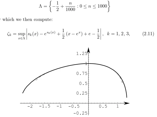
We deem meaningful to verify how the explicit approximations are related to the invariant (2.6). For that purpose the interval
−12,12
, which includes the origin, is discretized into 1000 subintervals. Hence we obtain the finite set:
for which we then compute:
ζk = sup
obtaining: 3
ζ2= 4.04683×10⁻⁵, ζ3= 4.53918×10⁻⁷, ζ4= 4.0769×10⁻⁹,
and this estimation is better than (2.7) concerning the solution (x(t), y(t)) obtained by means of the usual numerical methods. Figure 4 gives a pictorial view of this, showing the explicit approximations2(x) (dotted line) ands4(x)
(continuous line).
A fair objection that could be raised is that, when testing (2.7), one must sample the whole orbit, whilst our computation ofζk took place on a strictly
local basis. Accordingly, let us perform a new computation defining ∆1 and
∆2 as:
Note that the comparison is significant because the simulation shows that
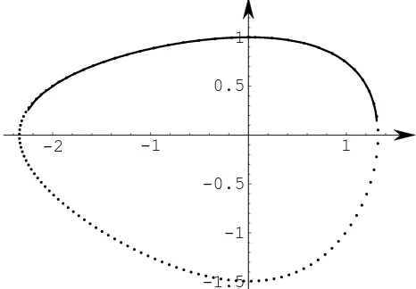
x(t)∈
the first integral better than the numerical solutions do. The final figure gives the complete Mathematicar solution (x(t), y(t)) as a dotted line versus the
s4(x) plotted with a continuous line forx∈[−2.30,1.309].
3
-2 -1 1
-1.5 -1 -0.5 0.5 1
Figure 5: s4versus the Mathematicar numerical solution.
3
Asymptotic approximations
It should be clear up to now that, even if the theoretical ground for ap-proximating the explicit solution of the Lotka-Volterra (or other hamiltonian) equations is the Dini theorem, nevertheless only the algebraic track has been led for doing the explicitation. Beyond its remarkable outsets, it has a severe boundary in its own nature, being possible to write it only till the fourth order.
In this section we present a meaningful improvement to obtain once again a closed form, but more accurate approximations of the Lotka-Volterra problem on the phase plane. Following closely the proof of Theorem 1, we will obtain the explicit solution of the equationh(y) =g(x) through the series reversion method applied to a Taylor polynomial of the functionh(y).
The loss of accuracy due to the fact we cannot write forn≥5 the exact solution of the approximate equation:
pn(y, y0) =
n
X
k=0 h(n)(y
0)
n! (y−y0)
k
=g(x),
is balanced by the better accuracy forh(y) that one can achieve increasing the Taylor’s polynomial degree. E.g. in the test case previously seenh(y) =y−ey
withy ∈[0,1],putting:
Θ =n n
2000 : 0≤n≤2000
we have:
Of course the reversion doesn’t settle the function that, according to the pre-vious sections, we call sn(x)—which, generally speaking, will be a
transcen-dental function ofx—but thenth order Taylor polynomial relevant to such a
function, and we note it asrn(x). The reverse series shall then be computed
forg(x),which, in the test case isg(x) = 1
by a computer Macintosh G4 with clock rated at 733 MHz, bus of 133 MHz and 640 MB RAM, has been of 0.7 seconds:
r8(x) = 1−
Up to this point we can computeζ8, see (2.11), namely the figure
appre-ciating the accuracy of the asymptotic solution versus the first integral:
where the discrete set Λ has the same meaning of the previous section. With a time machine of 0,05 seconds we will appreciate an accuracy improvement:
ζ8= 3.10769×10⁻¹¹.
We put our reversion till tor22(x), even if in such a case the elapsed time was
14617 seconds, but the accuracy is:
ζ22= 8.88178×10⁻¹⁶,
the same even doubling the discretization step. Last, the range ofxby
in which it has been checked that
max
Then, even if the broadening of the sample range makes worse the accuracy, such an approximation keeps its validity till to the tenth digit for the 54% of the solution existence range.
Last we compare the highest algebraic approximations4(x) with the
asymp-totic approximation r4(x). The asymptotic solution’s accuracy is obviously
less, but not immensely less:
max
and the distance beween them will be not greater than:
max
x∈Λ|s4(x)−r4(x)|= 4.18236×10 −7
4
Conclusions
We obtained an explicit solution of Lotka-Volterra equations founded upon the existence of its first integral holding a couple of phase variables (x, y) inextricably tied.
We started with a Taylor’s power expansion in the variabley. Truncating the expansion to the fourth term, we can use the machinery of classical algebra in order to solve for y. This algebraic approximation has been proved to be better than the highly accurate predictor/corrector numerical procedures. Our benchmark is in any case based on the approximate solutions capability to satisfy the first integral.
The above approximation can be improved (asymptotic approximation) taking more terms beyond the fourth in the Taylor expansion, and inverting fory. This approximation is by far more accurate than the algebraic one.
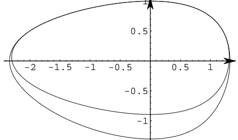
Nothing has been told hitherto about the approximate solution’s domain. This problem is too involved for being solvable in its generality: therefore we will provide an overview of it treating some concrete cases. In order to do this the hamiltonian of the original system, depending ony, is replaced by some Taylor approximation. Doing so, we succeed in calculating the (approximate) explicit equation of its integral curve. Its range of existence is then determined by the crossings of the relevant orbit with the horizontal axis. E. g. the closed curve of equation (2.6) has been pictured by the line of equation
1 2 +
x−ex
2 + (1−e) (y−1)−
e(y−1)2
2 −
e(y−1)3
6 −
e(y−1)4 24 = 0,
which we use for calculating s4(x), and then capable of approximating the
solution for y >0.
In such a way, with a numerical approach, we can see that puttingy= 0,
(2.6) givesx≃ −2.34026 andx≃1.32477, while the approximate hamiltonian cuts the xaxis atx≃ −2.29732 andx≃1.31062.
-2 -1.5 -1 -0.5 0.5 1
-1 -0.5 0.5 1
Figure 6: The exact (outer) and the approximate (inner) orbits.
Of course, increasing thenth-approximation order, the approximant orbit becomes closer and closer to the original one: in such a way for n= 8 the ap-proximate curve crosses atx≃ −2.34025 andx≃1.32477, almost the same as the original orbit. The highest absolute difference between the hamiltonians, the exact one and the 8th order approximation, fory >0 is 6.8046×10⁻⁶.
Both approaches to simulate the first integrals by means of Taylor polyno-mials seem quite viable but, as far as we know, they have not been attempted before, probably due to prohibitive computations. In any case, our method’s effectiveness is by large extent due to the computer algebra systems.
The algebraic approximations, by which we succeeded in calculating long arcs of the orbit on the population plane (x, y) for the Lotka-Volterra system, leads to very complicated integrals, as a right hand side of the so calledtime equation. Let us take, for example, the first equation from system (2.5):
˙
x(t) = 2 (1−expy(t)),
and set the initial conditionx(0) = 0. Replacingy(t) with one of the approx-imationsk(x), in the easiest casek= 2 we obtain:
t=1 2
Z x
0
dξ
1−exp 1 +
p
1−e(1−e+ expξ−ξ)
e
!.
Acknowledgments
We couldn’t close our paper without expressing our gratitude and thanks to Dr. Allan Hayes (http://www.haystack.demon.co.uk) who very promptly and courteously helped us put Mathematicar to work computing orbits and
generating plots, as well as adding to them the arrows denoting the direction in which axes increase.
We are also indebted with James Goebel Junghanns who helped us in the text formal revue.
References
[1] Knapp, R., Wagon, S., Check, Your Answers. . . But How?, Mathematica Edu. Res.,7(1998) no.4, 76–85
[2] Knopp, K., Theory and Application of Infinite Series, Blackie, London, 1928, reprinted by Dover, New York, 1990.
[3] Mingari, G., Ritelli, D. A Historical Outline of the Theorem of Implicit Functions, Divulg. Mat.10(2) (2002), 171–180.