Transmission of Economic Status
Changed?
Susan E. Mayer
Leonard M. Lopoo
A B S T R A C T
Only a few studies have tried to estimate the trend in the elasticity of chil-dren’s economic status with respect to parents’ economic status, and these studies produce conflicting results. In an attempt to reconcile these findings, we use the Panel Study of Income Dynamics to estimate the trend in the elas-ticity of son’s income with respect to parental income. Our evidence suggests a nonlinear trend in which the elasticity increased for sons born between 1949 and 1953, and then declined for sons born after that. Thus depending on the time periods one compares, the trend could be upward, downward, or flat. This and other factors help explain the different estimates for the trend in mobility.
I. Introduction
The extent to which economic status is transmitted from one genera-tion to the next has long been of interest to social scientists and policy makers largely because of the belief that the intergenerational transmission of economic status vio-lates norms of equal opportunity. Many studies have estimated the elasticity of son’s
Susan E. Mayer is dean and an associate professor at the Irving B. Harris Graduate School of Public Policy Studies and at the College at the University of Chicago. Leonard M. Lopoo is an assistant professor of public administration at the Maxwell School of Citizenship and Public Affairs at Syracuse University. The authors wish to thank Thomas DeLeire, Angela Fertig, Christopher Jencks, Helen Levy, Darren Lubotsky, Douglas Wolf, three anonymous referees, and participants in seminars at the University of Chicago and Harvard University as well as participants in a conference sponsored by Statistics Canada in Ottawa in February, 2001 for helpful comments and suggestions. Lopoo thanks the Bendheim-Thoman Center for Research on Child Wellbeing and the Office of Population Research, which is supported by cen-ter grant 5 P30 HD32030 from NICHD, at Princeton University for financial support. An earlier version of this paper was also presented at the 2000 Canadian International Labor Network conference. The data used in this article can be obtained beginning October 2005 through September 2008 from Leonard Lopoo, 426 Eggers Hall, Syracuse University, Syracuse, NY 13244, <lmlopoo@maxwell.syr.edu> [Submitted November 2001; accepted February 2004]
ISSN 022-166X E-ISSN 1548-8004 © 2005 by the Board of Regents of the University of Wisconsin System
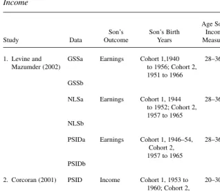
economic status with respect to father’s economic status in the United States (see Solon 1999 for a review of these studies), and the consensus today is that this elastic-ity is around 0.4 (Solon 1992, 1999). However, only four studies have estimated the trend in the elasticity of sons’ income or earnings with respect to parents’ income. Table 1 summarizes the nine estimates from these four studies.1Four of the nine esti-mates show that the elasticity increased, four show that it decreased, and one shows that it stayed the same. This paper produces new estimates of the trend that improve on earlier work and tries to reconcile these new estimates with the disparate findings from previous research.
All the studies in Table 1 compare elasticities for cohorts (two, four, or five) that were selected because of data availability rather than theoretical concerns and the time period over which the elasticity is measured depends on the data. If the trend in the elasticity changes over time in a nonmonotonic way, the choice of endpoints can affect the conclusion about the direction of the trend. The studies also differ in other ways that could result in different conclusions about the trend in the elasticity of son’s income (or earnings) with respect to parents’ income, including the data set, whether all sons or only sons in married-couple families are included, how parental income is measured, and the age at which son’s economic status is measured.
Several studies show that intergenerational occupational mobility increased for cohorts born from around 1900 to 1965 (Biblarz, Bengslan, and Bucur 1996; Grusky and DiPrete 1990; Hauser and Featherman 1977; Hout 1988).2We know of no study that shows a decline in intergenerational occupational mobility. Occupational mobil-ity is usually measured as the extent to which parents and their children are in occu-pations with the same level of “prestige” or socioeconomic standing. Prestige ratings depend on survey respondents’ or experts’ rating of occupations. The socioeconomic standing of an occupation is usually measured as a composite of the income and education characteristics of the people who hold the occupation. The correlation between father’s and son’s occupational socioeconomic ratings is greater than the correlation when prestige ratings are used (Jencks 1990). The correlation between father’s and son’s occupational socioeconomic status is in the range of 0.35 to 0.45, which is similar to the intergenerational correlation of father’s and son’s income, earnings, and wages when these are averaged over several years (Solon 1999;
1. Hauser (1998) also estimates the trend in the elasticity using the Occupational Change in a Generation Survey for 1962 and 1973. However, the sons in the youngest cohort in these data were born in 1939–48, which is the age range of the oldest sons used for the estimates in Table 1. Hauser estimates that mobility increased for nonblack men between these two surveys. Hauser also estimates elasticities using the 1986–88 Survey of Income and Program Participation. However, to estimate a trend in the elasticity in cross-sectional data such as these, one must compare elasticities for cohorts of sons who are different ages. As we discuss below, age and time could be confounded in these estimates.
Zimmerman 1992). If, as some researchers (see especially, Hauser 1998; Zimmerman 1992) argue, occupation is a proxy for permanent income, these studies suggest an increase in economic mobility for cohorts born in the first half of the last century.
Like previous research on intergenerational mobility, we are mainly interested in the stylized facts, so we do not try to explain the trend or test a particular theory about the trend. However, because the believability of stylized facts is strengthened when they correspond to theoretical predictions, in the final section of the paper we discuss recent theoretical predictions regarding the trend in economic mobility.
We estimate the elasticity of a son’s own family income measured when he is 30 years old with respect to the income of his parents when he was growing up. In Table 1
Estimates of the Elasticity of Son’s Earnings or Income with Respect to Parents’ Income
Age Son’s Elasticity Son’s Son’s Birth Income Cohort 1 to Study Data Outcome Years Measured Cohort 2
1. Levine and GSSa Earnings Cohort 1,1940 28–36 0.115 to 0.491 for Mazumder (2002) to 1956; Cohort 2, sons from
1951 to 1966 married parents;
GSSb 0.168 to 0.662*for
all sons NLSa Earnings Cohort 1, 1944 28–36 0.229 to 0.391**
to 1952; Cohort 2, for sons from 1957 to 1965 married parents;
NLSb 0.235 to 0.330 for
all sons PSIDa Earnings Cohort 1, 1946–54, 28–36 0.452 to 0.289 for
Cohort 2, sons from 1957 to 1965 married parents;
PSIDb 0.365 to 0.286 for
all sons 2. Corcoran (2001) PSID Income Cohort 1, 1953 to 20–30 0.26 to 0.18 (no
1960; Cohort 2, test of 1961 to 1968 significance) 3. Hauser (1998) GSS Imputed Four cohorts born 25–64 No trend
income 1922 to 1963 (nonblack
men)
4. Fertig (2003)a PSID Earnings Five cohorts born 21–40 0.500 to 0.217*
1945 to 1972 (difference between Cohort 1 and Cohort 5)
Notes: **p< 0.01; *p< 0.05
both generations family income includes labor income and cash income from all sources for all members of the family. We use son’s income rather than his earn-ings or wages as a measure of his economic status for two reasons. First, by using son’s family income we can include sons who are not working so long as they have another source of family income such as spouse’s earnings. Second, most studies of intergenerational economic mobility adopt the logic of the human capital model, which implies that parental investments increase children’s human capital, which then increases the child’s wages and earnings. But human capital also affects chil-dren’s success in the marriage market (Mare 1991; Pencavel 1998), and it might affect nonlabor income such as income from investments. Parental investments also might affect characteristics of children other than their human capital that in turn affect their success in the marriage market. Because a son’s family income is the result not only of his endowments and parental investment, but also his deci-sions about how many hours to work and his living arrangements, trends in the relationship between parental income and son’s income may not be the same as trends in the relationship between parental income and son’s wages or earnings if, for example, the correlation between sons’ earnings and their spouse’s earnings changes over time.
We use parental income rather than father’s wages or earnings as our measure of parents’ economic status because parental income is a better proxy for the invest-ments that can be made in the child and because it allows us to include sons who do not live with their father. Using parents’ income rather than father’s wages or earn-ings to predict son’s income also allows us to take into account changes in mother’s work effort on son’s future income. As more mothers work, the investments that fam-ilies can make depends less on just father’s earnings and more on family income (Harding et al. 2005).
II. Data and Methods
The Panel Study of Income Dynamics (PSID) is a longitudinal data set initiated with a core sample of approximately 4,800 families in 1968.3When chil-dren in the original sample established their own households, they and all members of their new household were included in the data set, thereby increasing the sample size over time. Our PSID sample includes all males born between 1949 and 1965 whose parents were respondents to the PSID and who had positive family income when they were 30 years old, although the income could come from sources other than the son’s earnings such as spouse’s earnings or unearned income.4The structure of the PSID implies that these men were heads of household when they were 31.
One potential cause for concern in longitudinal data is sample attrition. Fitzgerald, Gottschalk, and Moffitt (1998) estimated the bias in intergenerational earnings
mobil-3. We use both the SRC and the SEO samples for these estimates. The SRC sample is nationally represen-tative of families in 1967. The SEO has an oversample of low-income families in 1967. We weight these cases to make them nationally representative.
ity estimates caused by sons who left the PSID sample. They found no statistically significant difference in the elasticity of son’s earnings with respect to father’s earn-ings between a sample that included both sons who eventually did and did not leave the sample and a sample of sons who eventually left the sample. Their findings apply to attrition of sons between 1977 and 1989. In principle, attrition of parents could also result in biased estimates of the elasticity. In practice income data was available for all but 4.8 percent of the parents of sons eligible to be in our sample so this is unlikely to be a large source of bias.
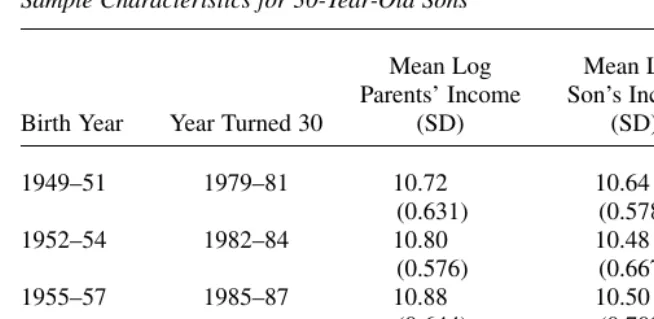
Table 2 describes our PSID sample by three- or four-year birth cohorts. As in pre-vious studies this choice of cohorts is guided by data rather than theoretical consid-erations, and we present this descriptive data by cohorts as a convenience. We defined cohorts to balance the number of years and number of cases in each cohort.5 Mean parental income increased over these cohorts but the mean of son’s income at age 30 decreased. Table 2 shows that the standard deviation of both son’s and par-ents’ income increased reflecting the well-documented increase in inequality over this time period.
To estimate the intergenerational elasticity of economic status, economists (see, for example, Mulligan 1997; Solon 1992) usually estimate the relationship between the logarithm of parent’s economic status (Yp) and the logarithm of children’s (Yc) economic status using the following equation:
( )1 lnYc=a+bplnYp+fc,
where εis a stochastic error term, the subscript cindicates the child and the sub-script pindicates the parents. In our case economic status is measured by family income in both generations so βpis the elasticity of a son’s income with respect to
his parents’ income. Ideally we would estimate the elasticity of son’s permanent income with respect to parental income averaged over all the years after a child was born in order to reduce error introduced by the transient component of income. Unfortunately, requiring so many years of parental income would result in a very small sample. To approximate permanent income, we average parental income over the years when a child was aged 19 to 25.6Families with less than three years of income were excluded in order to minimize error in the measurement of the parents’ permanent income.7Many studies show that using several years of parental income results in a higher elasticity than using only one year of parental income (see, for
5. We adjust all income values to 1995 dollars using the CPI-U-X1. This does not affect trends in the relationship between parents’ and son’s income.
example, Solon 1992; Zimmerman 1992). Mayer (1997) shows that in the PSID the elasticity of son’s earnings with respect to parental income measured in one year was 41 percent of the elasticity estimated when parental income is averaged over ten years. The elasticity when parental income was averaged over five years was 86 percent of the elasticity when parental income was averaged over ten years. Mazumder (2005) using data from the Survey of Income and Program Participation matched to the Social Security Administration’s earnings records, estimates that the elasticity of earnings for a pooled sample of sons and daughters with respect to their father’s earnings measured in one year was 55 percent of the elasticity estimated when fathers earnings were averaged over 10 years. The elasticity for father’s earn-ings averaged over ten years was 91 percent of the elasticity for father’s earnearn-ings measured over 15 years.8Thus our estimate using parental income averaged over seven years is probably not as large as a measure of the elasticity of permanent income. But for our purposes in estimating the trend in the elasticity, it is only important that the bias introduced by the transitory component of income be con-stant over time.
A measure of parental income when sons were younger than 19 to 25 might be a better proxy for the income that was available during the son’s childhood. The younger the age at which we measure parental income, the smaller the sample becomes, however. To see if measuring income at a younger age is likely to produce a
8. From Mazumder (2005), Table 5. Table 2
Sample Characteristics for 30-Year-Old Sons
Mean Log Mean Log
Parents’ Income Son’s Income Number of
Birth Year Year Turned 30 (SD) (SD) Cases
1949–51 1979–81 10.72 10.64 245
(0.631) (0.578)
1952–54 1982–84 10.80 10.48 317
(0.576) (0.667)
1955–57 1985–87 10.88 10.50 317
(0.644) (0.708)
1958–61 1988–91 10.86 10.50 375
(0.653) (0.766)
1962–65 1992–95 10.89 10.54 313
(0.699) (0.714)
Source: Authors’ calculations from PSID data described in text.
different estimate of the elasticity, we selected a subset of sons for whom we had fam-ily income measured both when they were 12 to 14 years old and when they were 19–25 years old. We used a Chow (1960) test to determine if the elasticities were the same when parental income was measured at these different ages and failed to reject the null hypothesis that the coefficients were the same.
Classical measurement error in son’s income should not bias the estimate of βp
(Levine and Mazumder 2002), although other sources of measurement error could cause bias in an unknown direction. Given the potential problems associated with measurement error, the potential bias from unobserved heterogeneity, as well as other potential problems associated with nonexperimental data, one should not interpret βp
as the causal influence of parental income.
Using Equation 1 we find that for all 30-year-old sons born between 1949 and 1965, the elasticity between parental income and son’s income is 0.34. This estimate is lower than the estimate of the intergenerational elasticity (0.48) obtained by Solon (1992, Table 4), and it is in the lower range of other studies that use the PSID and average parental income over several years. However, it is greater than the elasticity estimated by Corcoran (2001) and similar to the estimate from Levine and Mazumder (2002) using the PSID.
Because our emphasis is on the trend rather than the level of intergenerational mobility and estimating changes in mobility requires a different data structure, we do not try to reconcile our estimate of the overall elasticity with elasticities esti-mated in other studies. Nonetheless, recognizing a few differences between our estimate and Solon’s (1992) is useful because Solon’s estimates are the most widely cited using the PSID. Solon’s sample includes sons born between 1951 and 1959. When we confine our sample to sons born in these years, our elasticity rises to 0.39. We drop sons whose income was in the top 1 percent or bottom 1 percent of the income distribution to avoid the influence of outliers. Solon reports that excluding sons and fathers with annual earnings less than $1,000 (in 1967 dollars) reduces βp. Solon apparently uses unweighted data. Because our trends are
intended to be descriptive, we weight the data. βpis larger (0.36) when we use
unweighted data. While these differences affect the estimated level of intergenera-tional mobility, they are less likely to affect the estimated trend. Unlike Solon, we include sons whose fathers were not present in the home. When Solon includes sons from mother-headed families in his sample the elasticity decreases from 0.48 to 0.44. As we will see below, including sons from mother-only families can affect the trend as well as the level of mobility.9
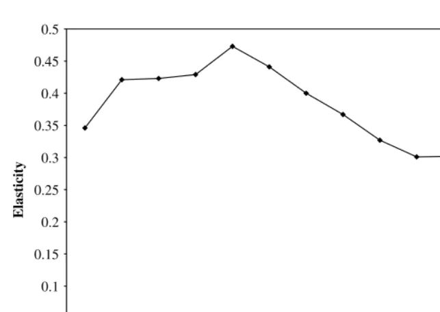
Figure 1 shows the trend in the elasticity of son’s income with respect to parental income estimated from Equation 1 using the entire sample. To smooth the trend, we divided the sample into 14 overlapping or “rolling” groups. Males born between 1949
9. There are other differences between our estimate and Solon’s estimate. Solon omits respondents who were part of the SEO, a survey component that overrepresented low-income families in 1967. We include these respondents. Solon reports that including respondents in this sample raises βp.Solon measured fathers’
and 1952 are Group 1. Males born between 1950 and 1953 are Group 2 and so on through males born in 1965. The estimated effect of parental income is thus a mov-ing average in which each individual appears up to four times. The data shown in Figure 1 is presented in Appendix Table A1.
Figure 1 shows that the elasticity of son’s income with respect to parents’ income first rose then declined. The elasticity peaks at 0.473 for children born between 1953 and 1956. It reaches its lowest level, 0.263, for children born between 1960 and 1963. We estimate the linear trend over the entire time period using the following model:
( )2 lnY lnY (lnY year* ) year ,
c=a+b p+c p +d 5+oc
where year is a continuous variable ranging from zero for sons born in 1949 to 16 for sons born in 1965. The coefficient for year (δ) tells us how son’s income changed over time. Because we control the time trend in son’s income, the coeffi-cient for the interaction (γ) tells us the change in the elasticity over time net of the time trend in son’s income. If γis statistically significant, the trend is significant. This model is comparable to a model that estimates a within-cohort elasticity and then compares the elasticities for different cohorts.10Thus our model is analogous Figure 1
to previous estimates except that we measure time by year rather than by cohort. The first column of Table 3 shows that the linear trend in the elasticity is negative (−0.008) but statistically insignificant.
III. Comparisons with Previous Research
Figure 1 suggests that an estimate of the trend in mobility that com-pares two cohorts will partly depend on the selection of the cohorts because the trend in the elasticity is not linear. Corcoran (2001) compares mobility for sons born in 1953–60 to sons born in 1961–68. This is the period over which the elasticity declined in Figure 1. Model 2 in Table 3 shows that the linear decline in the elasticity between 1953 and 1965 is statistically significant. So it is no surprise that Corcoran concludes that mobility increased.
When Levine and Mazumder use PSID data to compare sons born between 1946 and 1954 to sons born between 1957 and 1965, they find a statistically insignificant decrease in the elasticity from 0.452 to 0.289. When we use our sample to compute the elasticity for 30-year-old sons born between 1949 and 1954 (compared to Levine Table 3
OLS Estimates of the Elasticity of Son’s Income with Respect to Parental Income by Year of Birth and Parental Education
Model 3 Model 4
All Years, Sons All Years, Sons Model 2 whose Parents whose Parents Model 1 Sons Born have ≤12 Years have >12 Years
Predictor All Years 1953–65 of Schooling of Schooling
Log parental 0.412** 0.578** 0.447** 0.318
income (0.060) (0.107) (0.069) (0.172)
Log parental −0.008 −0.022* −0.012 −0.001
income*year (0.007) (0.010) (0.008) (0.017)
Year 0.077 0.245* 0.123 0.008
(0.071) (0.110) (0.086) (0.188)
R2 0.106 0.106 0.103 0.080
N 1,567 1,221 1,349 216
Source: PSID data described in text.
Notes: **p< 0.01; *p < 0.05; Model 1 estimates the relationship between the logarithm of parent’s income
(Yp) and the logarithm of children’s (Yc) income:
( ) ,
lnY lnY lnY*year year
c=a+b p+c p +d +oc
and Mazumder’s 1946 to 1954) and 1957 to 1965, the elasticity declines from 0.405 to 0.308, which is also statistically insignificant. Whether one believes that the elas-ticity remained the same or declined depends in part on the years over which the trend is measured.
Estimates of the trend in mobility also depend on whether they are for all sons or only for sons from married couple families. Our estimates and Corcoran (2001) include all sons regardless of the marital status of their parents. In their main results Levine and Mazumder (2002) omit sons from single-parent families because of data issues, but also because of concerns that income may be measured with more error for single parents and single parents may drop out of the sample more frequently than married parents. However, these results omit an increasingly large share of sons over time because the percentage of sons in single-parent fam-ilies increased. As Table 1 shows, when Levine and Mazumder reestimate the elas-ticities for a GSS sample that includes sons from single-parent families, the increase in the elasticity becomes larger and statistically significant. But Hauser (1998) finds no change in mobility in the GSS for a sample that includes sons from single-parent families. When Levine and Mazumder include all sons in the NLS the increase in the elasticity between the two cohorts diminishes and becomes sta-tistically insignificant. The decline in the elasticity in their PSID sample is statis-tically insignificant regardless of whether they include sons from mother-only families or not. Thus in some data sets the trend in the elasticity is sensitive to whether sons from single-parent families are included.
1966 cohort is compared to the 1979 cohort. To try to account for this possibility, Levine and Mazumder use data on a subset of fathers in the 1966 survey who reported their own income to correct the son’s income reports in that survey (although they do not describe the nature of the correction). Confidence in the change in the elasticity in NLS data therefore depends on confidence that this cor-rection accounts for all relevant differences in measurement error across the cohorts.11
The studies in Table 1 use different measures of son’s economic status (income or earnings). There is no particular reason that the trend in the elasticity of son’s earn-ings with respect to parents’ income should be the same as the trend in the elasticity of son’s income with respect to parents’ income. However, when we use our PSID sample to estimate the trend in the elasticity of son’s earnings with respect to parents’ income we find that the elasticity follows the same trend as the elasticity in Figure 1, first a rise and then a decline. Corcoran also finds the same trend whether son’s eco-nomic status is measured as labor income, hourly wages, or family income. Thus, we do not think that the difference in the measure of son’s economic status accounts for the difference in the elasticity across studies.
Previous research suggests that the elasticity is greater for older than for younger sons (Bowles and Gintis 2002). For example, Hauser (1998) reports that the elas-ticity of son’s income with respect to father’s imputed income is 0.169 for sons who are 25–34 years old, and 0.261 for sons who are 35–44 years old in 1993 to 1996.12 Thus in measuring the trend in the elasticity it is important that the mean age of the cohorts is the same over time. We measure son’s income at age 30. All the other studies in Table 1 include sons whose age falls within a several-year range. Corcoran measures sons’ income when they are age 25–27, which is a very short age range. As noted Hauser uses sons whose age falls within ten-year intervals. Hauser does not report the mean age within cohorts, so we cannot tell if the aver-age aver-age changes over time. Levine and Mazumder (2002) measure income for sons who are aged 28 to 36 years old. The mean age of sons is nearly identical in both cohorts of their NLS sample. But in their PSID sample, son’s age increases by almost two years from 28.75 years in the older to 30.71 years in the younger cohort. Thus the decline in the elasticity across these cohorts could be somewhat under-stated due to the increase in mean age.
IV. Sensitivity Tests
A key assumption of all estimates of the trend in mobility is that parental income is measured consistently over time. The PSID measure of parental
11. In the 1966 NLS family income is coded categorically while in 1979 it is continuous. Levine and Mazumder recode 1979 data to be consistent with the 1966 categories. Family income is continuous in all years of the PSID. We experimented with recoding PSID data into categories and found that this had little effect on the estimated elasticities. We also experimented with several alternative ways of top-coding the PSID data and found that this had little effect on the estimated elasticities. Levine and Mazumder also report that top-coding had little effect on their estimates.
income is likely to be more consistent than the measure from the NLS, the GSS or other survey data sets because the PSID is the only longitudinal data set that has asked relatively consistent questions about income over time. However, even when respon-dents are asked the same questions and reply with the same degree of accuracy, the quality of their responses can change over time. For example, the measure of parental income could become a less accurate indicator of permanent family income over time if, for example, parents were more likely to be retired in more recent cohorts because retirement income presumably is less representative of lifetime income than the income of current workers. But in our PSID sample the percentage of parents that are retired hardly changed: 15.3 percent of household heads in the oldest cohort were retired compared to 15.1 in the youngest cohort. The mean age of the head of the parents’ household also hardly changed over time.13
Our sample includes only sons who became heads of household by age 31. If the proportion of sons who are heads by age 31 changes over time, it could bias the trend in the elasticity. However, 82 percent of sons born in 1949–51 were identified as heads of household by age 31 compared to 86 percent of sons born in 1963–65. This sug-gests that a change in men’s likelihood of being a head of household is not likely to be a large source of error in our results.
V. Discussion and Conclusions
Our results suggest that the trend in the elasticity of son’s income with respect to parents’ income depends on what years one compares, whether all sons or only sons from married parents are included, and how parental income is measured. Using PSID data the elasticity increased for sons born from 1949 to 1953 and decreased for sons born from 1954 to 1963. These results are consistent with other research using PSID data. However, they are inconsistent with Levine and Mazumder’s NLS finding of a significant decline in mobility for sons from married parents and with Hauser’s (1998) finding of no change in mobility using GSS data.
An increase in intergenerational economic mobility for sons born after 1953 is con-sistent with the increase in occupational mobility found in several studies (Biblarz, Bengslan, and Bucur 1996; Grusky and DiPrete 1990; Hauser and Featherman 1977; Hout 1988). However, these studies also find an increase in intergenerational occupa-tional mobility for sons born before 1953 when our results suggest a decline in income mobility. Harding et al. (2005) use GSS data and rank occupations in terms of their educational requirements and mean income. They find that the effect of a one-point difference between two fathers’ occupations on their sons’ family income
declined for sons born between 1900 and 1945, but showed no clear trend after that, which is consistent with Hauser’s finding of no trend in mobility.
Solon (in press) has developed a model of intergenerational mobility in which the steady-state intergenerational income elasticity is a function of four key factors: the strength of the heritability of income-generating traits, the efficacy of investment in children’s human capital, the earnings return to human capital, and the progressivity of public investment in children’s human capital. (See also Mayer and Lopoo, in press, on the last point.) The implication is that, if intergenerational mobility increases it could be because the heritability of relevant traits decreased, human capital invest-ment became less productive, returns to human capital declined, or public investinvest-ment in human capital became more progressive.
Over the time period for which we have data, the heritability of traits is unlikely to have changed. We have little evidence on changes in the productivity of investments in children. But the returns to schooling increased during the 1980s and 1990s (Katz and Murphy 1992). If children from rich families are more likely to go to college, the increase in the returns to schooling would all else equal increase the elasticity of chil-dren’s income with respect to parents’ income, which would support Levine and Mazumder’s NLS results. However, Levine and Mazumder find that little of the increase in the elasticity is attributable to an increase in the intergenerational trans-mission of educational attainment or to the returns to schooling. Harding et al. (2005) also find little increase in the effect of parental education on children’s income. Thus the increase in the returns to schooling does not seem to have resulted in a decrease in mobility.
Cognitive skills affect earnings and are strongly correlated across generations. If the returns to cognitive skill have increased, we would expect a decline in economic mobility. Although there is agreement that cognitive skills contribute to earnings net of schooling (Bowles and Gintis 2002; Winship and Korenman 1999), evidence does not suggest that the return to cognitive skills net of schooling have increased. After reviewing all the relevant studies that they could find, Bowles, Gintis, and Osbourne (2001) concluded that the evidence provided, “no support for the hypothesis that the effect of cognitive scores on earnings increased secularly over the four decades cov-ered by our estimates” (p.1156). Many noncognitive skills that affect earnings also are correlated across generations (Bowles and Gintis 2002; Duncan et al. 2005). We have almost no evidence about whether these factors have become more or less important. However, Harding et al. (2005) find that between the 1970s and the 1990s the costs of being Black, Hispanic, and raised in the South all fell significantly, which, all else equal, would result in an increase in mobility. None of this proves that there were not important changes in the returns to human capital that could have reduced mobility. It does suggest the need for a great deal of additional research on this issue.
noth-ing else changed. In addition, government regulation of the labor market increased in the wake of the civil rights movement (DiPrete 1987; Dobbin and Sutton 1998; Leonard 1984). If this led to more meritocratic hiring and promotion patterns, inter-generational mobility would increase.
We know of no research that directly tests the hypothesis that government effort increased income mobility. If government effort influences mobility, we should see that mobility increased more for low-income than high-income children. We estimate the linear trend in mobility for sons born between 1949 and 1965 separately by parental education and find that mobility increased for sons whose parents had 12 years of schooling or less but hardly changed for sons whose parents had more than 12 years of schooling, although neither estimate is statistically significant. Grusky and DiPrete (1990) find that greater government spending on the Equal Employment Opportunity Commission and on manpower and job training programs was associated with greater occupational mobility. They also argue that the rate of increase in occupational mobility slowed as the federal government’s efforts to pro-mote equal employment opportunity slowed in the early 1980s (when the youngest cohorts in our PSID sample, for whom the increase in mobility appears to slow or even reverse, entered the labor market). This evidence suggests the need for more research on importance of government effort to economic mobility.
Because the measure of income is consistent for both sons and parents and of high-quality over time in the PSID, it is probably the best source to estimate the trend in intergenerational mobility. But the trend in son’s mobility in the PSID is not monoto-nic over time and because the time period is short and the sample sizes small it is dif-ficult to draw strong conclusions about the direction of the trend, much less the cause of any changes in mobility. It is clear that only when we have additional data over a longer period of time will we be able to estimate the trend in intergenerational economic mobility with confidence.
Appendix
Data DescriptionWe select all individuals born between 1949 and 1965 who had parents in the PSID and had positive income when they were 30 years old. This sample includes 30-year-olds who attrited at any point between 1983 and 1995. For the attriters, we use the core weight assigned in the last year they were in the PSID (Hill 1992). To link these individuals to their mothers, we use the Parent Identification File.
Variable definitions
Son’s income is total family income for sons who head their own household inflated to 1995 dollars using the CPI-U-X1.
Parents’ education is the number of years of education the mother completed when her son was 19 years old. When this value was missing we used mother’s education in the first available subsequent year up to the time when the son was 25 years old. If mother’s education was still missing, we used the education of the father reported when the son was 25 years old.
Table A1
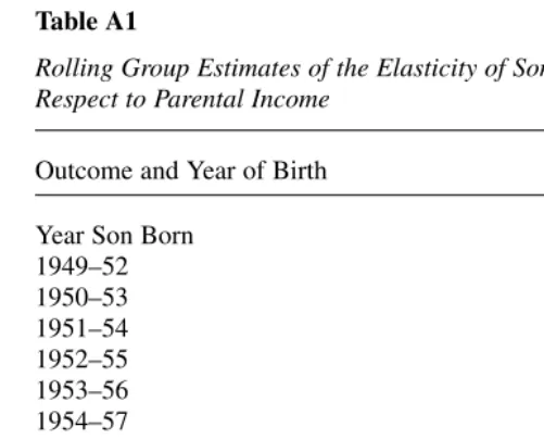
Rolling Group Estimates of the Elasticity of Son’s Income with Respect to Parental Income
Outcome and Year of Birth βp[t-statistic]
Year Son Born
1949–52 0.346 [5.59]
1950–53 0.421 [6.92]
1951–54 0.423 [6.88]
1952–55 0.429 [6.27]
1953–56 0.473 [6.50]
1954–57 0.441 [6.46]
1955–58 0.400 [5.91]
1956–59 0.367 [6.57]
1957–60 0.327 [6.08]
1958–61 0.301 [5.00]
1959–62 0.302 [5.07]
1960–63 0.263 [4.11]
1961–64 0.270 [3.88]
1962–65 0.279 [4.22]
Source: PSID data described in text and appendix.
Note: βpis the estimated relationship between the logarithm of parent’s income (Yp) and the logarithm of children’s (Yc) income using the following equation:
, lnYc=a+bplnYp+fc
where εis a stochastic error term, the subscript cindicates the child and the subscript p indicates the parents.
References
Biblarz, Timothy J., Vern L. Bengslan, and Alexander Bucur. 1996. “Social Mobility Across Three Generations.” Journal of Marriage and the Family58(1):188–200.
Bowles, Samuel, and Herbert Gintis. 2002. “The Inheritance of Inequality.” Journal of Economic Perspectives16(3):3–30.
Corcoran, Mary. 2001. “Mobility, Persistence, and the Consequences of Poverty for Children: Child and Adult Outcomes.” In Understanding Poverty, ed. Sheldon Danziger and Robert Haveman, 127–61. New York: Russell Sage Foundation.
Chow, Gregory C. 1960. “Tests of Equality Between Sets of Coefficients in Two Linear Regressions.” Econometrica28(3):591–05.
DiPrete, Thomas. 1987. “The Professionalization of Administration and Equal Employment Opportunity in the U.S. Federal Government.” American Journal of Sociology
93(1):119–40.
Dobbin, Frank, and Frank R. Sutton. 1998. “The Strength of a Weak State: The Rights Revolution and the Rise of Human Resources Management Divisions.” American Journal of Sociology104(2):441–76.
Duncan, Greg, Ariel Kalil, Susan E. Mayer, Robin Tepper and Monique Payne. 2005. “The Apple Does Not Fall Far from the Tree.” In Unequal Chances: Family Background and Economic Success, ed. Samuel Bowles, Herbert Gintis, and Melissa Osbourne. Princeton: Princeton University Press.
Fertig, Angela R. 2003. “Trends in Intergenerational Earnings Mobility.” Princeton, N.J.: Center for Research on Child Wellbeing, Princeton University. Working Paper No. 01–23. Fitzgerald, John, Peter Gottschalk, and Robert Moffitt. 1998. “An Analysis of the Impact of
Sample Attrition on the Second Generation of Respondents in the Michigan Panel Study of Income Dynamics.” Journal of Human Resources33(2):300–44.
Grusky, David, and Thomas DiPrete 1990. “Recent Trends in the Process of Stratification.” Demography27(4):617–36.
Harding, David, Christopher Jencks, Leonard Lopoo, and Susan Mayer. 2005. “The Changing Effect of Family Background on the Incomes of American Adults” In Unequal Chances: Family Background and Economic Success, ed. Samuel Bowles, Herbert Gintis, and Melissa Osbourne. Princeton: Princeton University Press.
Hauser, Robert. 1998. “Intergenerational Economic Mobility in the United States: Measures, Differentials and Trends.” Madison: University of Wisconsin. Unpublished.
Hauser, Robert, and David Featherman. 1977. The Process of Stratification: Trends and Analysis. New York: Academic Press.
Hauser, Robert M., and John R. Warren. 1997. “Socioeconomic Indexes of Occupational Status: A Review, Update, and Critique.” In Sociological Methodologyed. Adrian E. Raftery, 177–298. Cambridge, Mass.: Basil Blackwell.
Hill, Martha S. 1992. The Panel Study of Income Dynamics: A User’s Guide. Newbury Park, Calif.: Sage Publications.
Hout, Michael 1988. “More Universalism, Less Structural Mobility: The American Occupational Structure in the 1980s.” American Journal of Sociology93(6):1358–400. Jencks, Christopher. 1990. “What Is the True Rate of Social Mobility?” In Social Mobility and
Social Structure, ed. Ronald L. Breiger, 103–30. New York: Cambridge University Press. Jencks, Christopher, Susan Mayer, and Joseph Swingle. 2004. “Who Has Benefited from
Economic Growth in the United States since 1969? The Case of Children.” In What Has Happened to the Quality of Life in Advanced Industrial Nations, ed. Edward Wolff. Northhampton, Mass.: Edward Elgar Publishing.
Katz, Lawrence F., and Kevin M. Murphy. 1992. “Changes in Relative Wages, 1963–1987: Supply and Demand Factors.” Quarterly Journal of Economics107(1):35–78.
Leonard, Johnathan S. 1984. “The Impact of Affirmative Action in Employment.” Journal of Labor Economics2(4):439–63.
Levine, David I., and Bhashkar Mazumder. 2002. “Choosing the Right Parents: Changes in the Intergenerational Transmission of Inequality—Between 1980 and the Early 1990s.” Chicago: Federal Reserve Bank of Chicago, Working Paper No. 2002–08.
Mayer, Susan E. 1997. What Money Can’t Buy: Family Income and Children’s Life Chances. Cambridge, Mass.: Harvard University Press.
Mayer, Susan E., and Leonard M. Lopoo. In press. “What Do Trends in the Intergenerational Earnings Mobility of Sons and Daughters Mean?” In Generational Income Mobility in North America and Europe, ed. Miles Corak. Cambridge: Cambridge University Press. Mazumder, Bhashkar. 2005. “Earnings Mobility in the United States: A New Look at
Intergenerational Inequality.” In Unequal Chances: Family Background and Economic Success, ed. Samuel Bowles, Herbert Gintis, and Melissa Osbourne. Princeton: Princeton University Press.
Mueller, Charles W. and Hallowell Pope. 1980. “Divorce and Female Remarriage Mobility: Data on Marriage Matches after Divorce for White Women.” Social Forces58(3):726–38. Mulligan, Casey B. 1997. Parental Priorities and Economic Inequality. Chicago: University
of Chicago Press.
Pencavel, John. 1998. “Assortative Mating by Schooling and the Work Behavior of Wives and Husbands.” American Economic Review88(2):326–29.
Solon, Gary. 1992. “Intergenerational Income Mobility in the United States.” American Economic Review82(3):393–408.
———. 1999. “Intergenerational Mobility in the Labor Market.” In Handbook of Labor Economics, Volume 3,ed. Orley Ashenfelter and David Card, 1761–800. Amsterdam: North-Holland.
———. In Press. “A Model of Intergenerational Mobility Variation over Time and Place.” In Generational Income Mobility in North America and Europe, ed. Miles Corak. Cambridge: Cambridge University Press.
Winship, Christopher, and Sanders D. Korenman. 1999. “Economic Success and the Evolution of Schooling and Mental Ability” In Earning and Learning, ed. Susan E. Mayer and Paul E. Peterson. Washington, D.C.: Brookings Institution Press.