Dr. Kellie Mosley, Recent Medical School Graduate
“Calculus for the Utterly Confused has proven to be a wonderful review enabling me to move forward in application of calculus and advanced topics in mathematics. I found it easy to use and great as a reference for those darker aspects of calculus.”
Aaron Landeville, Engineering Student
“I am so thankful for Calculus for the Utterly Confused! I started out clueless but ended with an A!”
Erika Dickstein, Business School Student
“As a non-traditional student one thing I have learned is the importance of material sup-plementary to texts. Especially in calculus it helps to have a second source, especially one as lucid and fun to read as Calculus for the Utterly Confused. Anyone, whether a math weenie or not, will get something out of this book. With this book, your chances of survival in the calculus jungle are greatly increased.”
Beginning French for the Utterly Confused Beginning Spanish for the Utterly Confused Chemistry for the Utterly Confused English Grammar for the Utterly Confused Financial Aid for the Utterly Confused Physics for the Utterly Confused Statistics for the Utterly Confused
New York Chicago San Francisco Lisbon London Madrid Mexico City Milan New Delhi San Juan Seoul
Singapore Sydney Toronto
for the
Utterly Confused
Second Edition
0-07-151119-9
The material in this eBook also appears in the print version of this title: 0-07-148158-3.
All trademarks are trademarks of their respective owners. Rather than put a trademark symbol after every occurrence of a trademarked name, we use names in an editorial fashion only, and to the benefit of the trademark owner, with no intention of infringement of the trademark. Where such designations appear in this book, they have been printed with initial caps.
McGraw-Hill eBooks are available at special quantity discounts to use as premiums and sales promotions, or for use in corporate training programs. For more information, please contact George Hoare, Special Sales, at george_hoare@ mcgraw-hill.com or (212) 904-4069.
TERMS OF USE
This is a copyrighted work and The McGraw-Hill Companies, Inc. (“McGraw-Hill”) and its licensors reserve all rights in and to the work. Use of this work is subject to these terms. Except as permitted under the Copyright Act of 1976 and the right to store and retrieve one copy of the work, you may not decompile, disassemble, reverse engineer, reproduce, modify, create derivative works based upon, transmit, distribute, disseminate, sell, publish or sublicense the work or any part of it without McGraw-Hill’s prior consent. You may use the work for your own noncommercial and personal use; any other use of the work is strictly prohibited. Your right to use the work may be terminated if you fail to comply with these terms.
THE WORK IS PROVIDED “AS IS.” McGRAW-HILL AND ITS LICENSORS MAKE NO GUARANTEES OR WAR-RANTIES AS TO THE ACCURACY, ADEQUACY OR COMPLETENESS OF OR RESULTS TO BE OBTAINED FROM USING THE WORK, INCLUDING ANY INFORMATION THAT CAN BE ACCESSED THROUGH THE WORK VIA HYPERLINK OR OTHERWISE, AND EXPRESSLY DISCLAIM ANY WARRANTY, EXPRESS OR IMPLIED, INCLUDING BUT NOT LIMITED TO IMPLIED WARRANTIES OF MERCHANTABILITY OR FITNESS FOR A PARTICULAR PURPOSE. McGraw-Hill and its licensors do not warrant or guarantee that the functions contained in the work will meet your requirements or that its operation will be uninterrupted or error free. Neither McGraw-Hill nor its licen-sors shall be liable to you or anyone else for any inaccuracy, error or omission, regardless of cause, in the work or for any damages resulting therefrom. McGraw-Hill has no responsibility for the content of any information accessed through the work. Under no circumstances shall McGraw-Hill and/or its licensors be liable for any indirect, incidental, special, punitive, consequential or similar damages that result from the use of or inability to use the work, even if any of them has been advised of the possibility of such damages. This limitation of liability shall apply to any claim or cause whatsoever whether such claim or cause arises in contract, tort or otherwise.
We hope you enjoy this
McGraw-Hill eBook! If
you’d like more information about this book,
its author, or related books and websites,
please click here.
About the Authors
◆◆◆◆◆◆◆◆◆◆◆◆◆◆◆◆◆
DRROBERTOMANreceived the B.S. degree from Northeastern University and the Sc.M. and Ph.D. degrees from Brown University, all in physics. He has taught mathematics and physics at several col-leges and universities including University of Minnesota, Northeastern University, University of South Florida, and University of Tampa. He has also done research for Litton Industries, United Technologies, and NASA, where he developed the theoretical model for the first pressure gauge sent to the moon. He is author of numerous technical articles, books, and how-to-study books, tapes, and videos.
DR DANIEL OMAN received the B.S. degree in physics from Eckerd College. He received both his M.S. degree in physics and his Ph.D. in electrical engineering from the University of South Florida where he taught many utterly confusedstudents in classes and one-on-one. He has authored several books and technical articles and has also done research on CO2 lasers and solar cells. Dan has
spent ten years in the semiconductor manufactur-ing industry with AT&T Bell Labs, Lucent Technologies, and Agere Systems.
vii
◆◆◆◆◆◆◆◆◆◆◆◆◆◆◆◆◆
Contents
◆◆◆◆◆◆◆◆◆◆◆◆◆◆◆◆◆
A Special Message xi How to Study Calculus xiii
Preface xv
Chapter 1 Mathematical Background 1 1-1 Solving Equations 2 1-2 Binomial Expansions 4 1-3 Trigonometry 5 1-4 Coordinate Systems 6 1-5 Logarithms and Exponents 8 1-6 Functions and Graphs 10 1-7 Conics 16 1-8 Graphing Trigonometric Functions 23 Test Yourself 27 Answers 28
Chapter 3 Derivatives 41 3-1 Polynomials 43
3-2 Product and Quotient Rule 48
3-3 Trigonometric Functions 49
3-4 Implicit Differentiation 50
3-5 Change of Variable 52
3-6 Chain Rule 53
3-7 Logarithms and Exponents 55
3-8 L’Hopital’s Rule 56
Test Yourself 58
Answers 58
Chapter 4 Graphing 61
Guidelines for Graphing with Calculus 72
Test Yourself 77
Answers 77
Chapter 5 Max-Min Problems 81
Guidelines for Max-Min Problems 84
Test Yourself 90
Answers 91
Chapter 6 Related Rate Problems 95
Test Yourself 108
Answers 109
Chapter 7 Integration 113
7-1 The Antiderivative 114
7-2 Area Under the Curve 123
7-3 Average Value of a Function 135
7-4 Area between Curves Using dy 139
Test Yourself 143
Chapter 8 Trigonometric Functions 147
8-1 Right Angle Trigonometry 148
8-2 Special Triangles 152
8-3 Radians and Small Angles 154
8-4 Non-Right Angle Trigonometry 156
8-5 Trigonometric Functions 160
8-6 Identities 162
8-7 Differentiating Trigonometric Functions 166
8-8 Integrating Trigonometric Functions 170
Test Yourself 175
Answers 176
Chapter 9 Exponents and Logarithms 179
9-1 Exponent Basics 180
9-2 Exponential Functions 181
9-3 The Number e 186
9-4 Logarithms 191
9-5 Growth and Decay Problems 195
9-6 The Natural Logarithm 202
9-7 Limited Exponential Growth 203
9-8 The Logistic Function 212
Test Yourself 215
Answers 216
Chapter 10 More Integrals 221
10-1 Volumes 222
10-2 Arc Lengths 226
10-3 Surfaces of Revolution 228
10-4 Techniques of Integration 229
10-5 Integration by Parts 236
10-7 Integrals from Tables 242
10-8 Approximate Methods 243
Test Yourself 249
Answers 249
Mathematical Tables 253
xi
A Special Message to
the Utterly Confused
Calculus Student
◆◆◆◆◆◆◆◆◆◆◆◆◆◆◆◆◆
Our message to the utterly confused calculus student is very simple: You don’t have to be confused anymore.
We were once confused calculus students. We aren’t confused anymore. We have taught many utterly confused calculus students both in formal class set-tings and one-on-one. All this experience has taught us what causes confusion in calculus and how to eliminate that confusion. The topics we discuss here are aimed right at the heart of those topics that we know cause the most trouble. Follow us through this book, and you won’t be confused anymore either.
Anyone who has taught calculus will tell you that there are two problem areas that prevent students from learning the subject. The first problem is a lack of algebra skills or perhaps a lack of confidence in applying recently learned algebra skills. We attack this problem two ways. One of the largest chapters in this book is the one devoted to a review of the algebra skills you need to be successful in working calculus problems. Don’t pass by this chapter. There are insights for even those who consider themselves good at algebra. When we do a problem we take you through the steps, the calculus steps and all those pesky
little algebra steps, tricks some might call them. When we give an example it is a complete presentation. Not only do we do the problem completely but also we explain along the way why things are done a certain way.
The second problem of the utterly confused calculus student is the inability to set up the problems. In most problems the calculus is easy, the algebra possibly tedious, but writing the problem in mathematical statements the most difficult step of all. Translating a word problem into a math problem (words to equa-tion) is not easy. We spend time in the problems showing you how to make word sentences into mathematical equations. Where there are patterns to problems we point them out so when you see similar problems, on tests perhaps, you will remember how to do them.
xiii
How to Study Calculus
◆◆◆◆◆◆◆◆◆◆◆◆◆◆◆◆◆
Calculus courses are different from most courses in other disciplines. One big difference is in testing. There is very little writing in a calculus test. There is a lot of mathematical manipulation.
In many disciplines you learn the material by reading and listening and demon-strate mastery of that material by writing about it. In mathematics there is some reading, and some listening, but demonstrating mastery of the material is by doing problems.
For example there is a great deal of reading in a history course, but mastery of the material is demonstrated by writing about history. In your calculus course there should be a lot of problem solving with mastery of the material demon-strated by doing problems.
In your calculus course, practicing working potential problems is essential to success on the tests. Practicing problems, not just reading them but actually writing them down, may be the only way for you to achieve the most modest of success on a calculus test.
To succeed on your calculus tests you need to do three things, PROBLEMS, PROBLEMS, and PROBLEMS. Practice doing problems typical of what you expect on the exam and you will do well on that exam. This book contains explanations of how to do many problems that we have found to be the most confusing to our students. Understanding these problems will help you to understand calculus and do well on the exams.
General Guidelines for Effective
Calculus Study
1. If at all possible avoid last minute cramming. It is inefficient.
2. Concentrate your time on your best estimate of those problems that are going to be on the tests.
3. Review your lecture notes regularly, not just before the test.
4. Keep up. Do the homework regularly. Watching your instructor do a prob-lem that you have not even attempted is not efficient.
5. Taking a course is not a spectator event. Try the problems, get confused if that’s what it takes, but don’t expect to absorb calculus. What you absorb doesn’t mat-ter on the test. It is what comes off the end of your pencil that counts.
6. Consider starting an informal study group. Pick people to study with who study and don’t whine. When you study with someone agree to stick to the topic and help one other.
Preparing for Tests
1. Expect problems similar to the ones done in class. Practice doing them. Don’t just read the solutions.
2. Look for modifications of problems discussed in class. 3. If old tests are available, work the problems.
4. Make sure there are no little mathematical “tricks” that will cause you prob-lems on the test.
Test Taking Strategies
1. Avoid prolonged contact with fellow students just before the test. The nerv-ous tension, frustration, and defeatism expressed by fellow students are not for you.
2. Decide whether to do the problems in order or look over the entire test and do the easiest first. This is a personal preference. Do what works best for you. 3. Know where you are timewise during the test.
4. Do the problems as neatly as you can.
Preface
◆◆◆◆◆◆◆◆◆◆◆◆◆◆◆◆◆
The purpose of this book is to present basic calculus concepts and show you how to do the problems. The emphasis is on problems with the concepts devel-oped within the context of the problems. In this way the development of the calculus comes about as a means of solving problems. Another advantage of this approach is that performance in a calculus course is measured by your ability to do problems. We emphasize problems.
This book is intended as a supplement in your formal study and application of calculus. It is not intended to be a complete coverage of all the topics you may encounter in your calculus course. We have identified those topics that cause the most confusion among students and have concentrated on those topics. Skill development in translating words to equations and attention to algebraic manipulation are emphasized.
This book is intended for the nonengineering calculus student. Those studying calculus for scientists and engineers may also benefit from this book Concepts are discussed but the main thrust of the book is to show you how to solve applied problems. We have used problems from business, medicine, finance, economics, chemistry, sociology, physics, and health and environmental sciences. All the problems are at a level understandable to those in different disciplines.
This book should also serve as a reference to those already working in the var-ious disciplines where calculus is employed. If you encounter calculus occa-sionally and need a simple reference that will explain how problems are done this book should be a help to you.
xv
It is the sincere desire of the authors that this book help you to better understand calculus concepts and be able to work the associated problems. We would like to thank the many students who have contributed to this work, many of whom started out utterly confused, by offering suggestions for improvements. Also we would like to thank the people at McGraw-Hill who have confidence in our approach to teaching calculus and support this second edition.
Robert M. Oman
St. Petersburg, Florida
Daniel M. Oman
for the
MATHEMATICAL
BACKGROUND
◆◆◆◆◆◆◆◆◆◆◆◆◆◆◆◆◆
You should read this chapter if you need to review or you need to learn about
➜
Methods of solving quadratic equations➜
The binomial expansion➜
Trigonometric functions––right angle trig and graphs➜
The various coordinate systems➜
Basics of logarithms and exponents➜
Graphing algebraic and trigonometric functions1
Some of the topics may be familiar to you, while others may not. Depending on the mathematical level of your course and your mathematical background, some topics may not be of interest to you.
Each topic is covered in sufficient depth to allow you to perform the mathe-matical manipulations necessary for a particular problem without getting bogged down in lengthy derivations. The explanations are, of necessity, brief. If you are totally unfamiliar with a topic it may be necessary for you to consult an algebra or calculus text for a more thorough explanation.
The most efficient use of this chapter is for you to do a brief review of the top-ics, spending time on those sections that are unfamiliar to you and that you know you will need in your course, and then refer to specific topics as they are encoun-tered in the solution to problems. Even if you are familiar with a topic review might “fill in the gaps” or give you a better insight into certain mathematical operations. With this reference you should be able to perform all the algebraic operations necessary to complete the problems in your calculus course.
1-1
Solving Equations
The simplest equations to solve are the linear equations of the form ax⫹b⫽0, which have as their solution . The next most complicated equations are the quadratics. The simplest quadratic is the type that can be solved by tak-ing square roots directly.
Example 1-1 Solve for x: .
Solution: Divide by 4, and then take the square root of both sides.
Both plus and minus values are legitimate solutions. The reality of the problem producing the equation may dictate that one of the solutions be discarded.
The next complication in quadratic equations is the factorable equation.
Example 1-2 Solve by factoring.
Solution: The solutions, the values
of that make each parenthesis equal to zero, and satisfy the factored equation, are and .x⫽3 x⫽ ⫺2
x
(x⫺ 3)(x⫹2)⫽ 0 1
x2⫺ x⫺ 6⫽ 0
x2⫺ x⫺ 6⫽0 4x2
4 ⫽ 36
4 1 x2⫽9 1 x⫽ ⫾3 4x2⫽36
If the quadratic cannot be solved by factoring, the most convenient solution is by quadratic formula, a general formula for solution of any quadratic equation in the form . The solution according to the quadratic formula is
Problems in your course should rarely produce square roots of negative num-bers. If your solution to a quadratic produces any square roots of negative numbers, you are probably doing something wrong in the problem.
Example 1-3 Solve by using the quadratic formula.
Solution: Substitute the constants into the formula and perform the opera-tions. Writing above the equation you are solving helps in identifying the constants and keeping track of the algebraic signs.
The quadratic formula comes from a generalized solution to quadratics known as “completing the square.” Completing the square is rarely used in solving quadratics. The formula is much easier. It is, however, used in certain calculus problems, so an explanation of the technique is appropriate. A completing the square approach is also used in graphing certain functions.
The basic procedure for solving by completing the square is to make the equation a perfect square, much as was done with the simple example, . Work with the and xcoefficients so as to make a perfect square of both sides of the equation and then solve by direct square root. This is best seen by example. Look first at the equation , which can be factored and has solu-tions of ⫺5 and ⫺1, to see how completing the square produces these solutions.
Example 1-4 Solve by completing the square.
Solution: The equation can be made into a perfect square by adding 4 to both
sides of the equation to read or , which, upon
direct square root, yields x⫹3⫽ ⫾2, producing solutions ⫺5 and ⫺1. (x⫹ 3)2⫽4
x2⫹ 6x⫹9⫽4
x2⫹ 6x⫹5⫽0 x2⫹ 6x⫹5⫽0 x2
4x2⫽36
x⫽ ⫺b ⫾ 2b
2⫺ 4ac
2a ⫽
⫹5⫾ 225⫺ 4(1)(3)
2(1) ⫽
5⫾ 213
2 ⫽4.30, 0.70
ax2⫹bx⫹c⫽ 0
x2⫺5x⫹ 3⫽ 0
ax2⫹bx⫹c⫽0
x2⫺ 5x⫹3⫽0
x⫽ ⫺b⫾ 2b2⫺4ac 2a
As you can imagine the right combina-tion of coefficients of and xcan make the problem awkward. Most calculus problems involving completing the square are not especially difficult. The general procedure for completing the square is the following:
• If necessary, divide to make the coef-ficient of the term equal to 1.
• Move the constant term to the right side of the equation.
• Take 1/2 of the xcoefficient, square it, and add to both sides of the equation. This makes the left side a perfect square and the right side a number.
• Write the left side as a perfect square and take the square root of both sides for the solution.
Example 1-5 Solve by completing the square.
Solution: Move the 1, the constant term, to the right side: . Add 1/2 of 4 (the coefficient of x) squared to both sides: x2⫹4x⫹4⫽4⫺1. The
left side is a perfect square and the right side a number: . Take
square roots for the solutions: or .
Certain cubic equations such as can be solved directly producing the sin-gle answer . Cubic equations with quadratic ( ) and linear (x) terms can be solved by factoring (if possible) or approximated using graphical techniques. Calculus will allow you to apply graphical techniques to solving cubics.
1-2
Binomial Expansions
Squaring is done so often that most would immediately write . Cubing is not so familiar but easily accomplished by
multiplying by to obtain .
There is a simple procedure for finding the power of . Envision a string of s multiplied together . Notice that the first term has coefficient 1 with araised to the power, and the last term has coefficient 1 with braised to the nthpower. The terms in between contain ato progressively
nth
(a⫹ b)n
(a⫹b)
(a⫹ b)
nth
a3⫹3a2b⫹ 3ab2⫹b3
(a⫹ b) (a2⫹ 2ab⫹ b2)
(a⫹ b)
a2⫹ 2ab⫹ b2
(a⫹ b)
x2 x⫽ 2
x3⫽ 8
x⫽ ⫺2⫹ 23, ⫺ 2⫺ 23
x⫹ 2⫽ ⫾23
(x⫹ 2)2⫽3
x2⫹4x⫽ ⫺1
x2⫹ 4x⫹1⫽ 0 x2
decreasing powers, , and bto progressively increasing pow-ers, 0, 1, 2, . . . The coefficients can be obtained from an array of numbers or more conveniently from the binomial expansion or binomial theorem
The factorial notation may be new to you. The definitions are 0!⫽1, 1! ⫽1, 2! ⫽2⋅ 1, 3! ⫽3⋅ 2⋅ 1, etc.
Use of the binomial expansion to verify is one of the suggested problems.
1-3
Trigonometry
The trigonometric relations can be defined in terms of right angle trigonometry or through their functions. The basic trigonometric relations, as they relate to right triangles, are shown in the box below.
(a⫹ b)3
(a⫹ b)n⫽ an
0! ⫹
nan⫺1
b
1! ⫹
n(n ⫺1)an⫺2b2
2! ⫹
c n,n⫺ 1,n⫺ 2, . . .
Graphs of the trigonometric relations are shown in Fig. 1-1.
Fig. 1-1 tanq = b/a
cosq = a/c
sinq = b/c Opposite (b) side from angle
Adjacent (a)
side to angle
Hypotenuse (c)
BASIC TRIGONOMETRIC FUNCTIONS
q
2p 2p
2p
tanq sinq
cosq p
p
p
q
The tangent function is also defined in terms of sine and cosine: .
Angles are measured in radians and degrees. Radian measure is a pure number, the ratio of arc length to radius to produce the desired angle. Figure 1-2 shows the relationship of arc length to radius to define the angle.
The relation between radians and degrees is .
Example 1-6 Convert rad to degrees and 270⬚to radians.
Solution: , ,
There are a large number of trigonometric identities that can be derived using geometry and algebra. Several of the more common are in the following box: 270⬚2prad
360⬚ ⫽
3p
2 rad⫽4.7rad
0.36rad 360⬚
2prad ⫽ 20.6⬚
p
6 rad
360⬚ 2prad⫽ 30⬚
p/6 and 0.36
2prad⫽ 360⬚ tanu⫽ sinu/cosu
1-4
Coordinate Systems
The standard two-dimensional coordinate system works well for most calculus problems. In working problems in two dimensions do not hesitate to arrange the coordinate system for your convenience. The x-coordinate does not have to be horizontal and increasing to the right. It is best, however, to maintain the
x-yorientation. With the fingers of the right hand pointed in the direction of
xthey should naturally curl in the direction of y.Positions in the standard right angle coordinate system are given with two numbers. In a polar coordinate sys-tem positions are given by a number and an angle. In Fig. 1-3 it is clear that any point (x, y) can also be specified by (r,u).
Fig. 1-2
TRIGONOMETRIC IDENTITIES
a2⫹b2⫽c2 sin2q ⫹ cos2q ⫽ 1
sinq⫽cos(90°⫺q) cosq ⫽ sin(90°⫺q)
sin(a⫾b)⫽sinacosb⫾cosasinb
cos(a⫾b)⫽cosacosb ⫿sinasinb
tan(a⫾b)⫽ tana⫾ tanb 17tana tanb
tanu⫽ 1
Rather than moving distances in mutually perpendicular directions, the rand locate points by moving a distance rfrom the origin along what would be the ⫹x direction, then rotating counterclockwise through an angle . The relationship between rectangular and polar coordinates is also shown in Fig. 1-3.
Example 1-7 Find the polar coordinates for the point (3, 4).
Solution: andu⫽ tan⫺1
(4/3)⫽53⬚
r⫽ 232⫹ 42⫽ 5
u
u
Example 1-8 Find the rectangular points for (3, 120°).
Solution: x⫽3 cos 120°⫽ ⫺1.5 andy⫽3 sin 120°⫽2.6
As a check, you can verify that (⫺1.5)2⫹2.62⫽32.
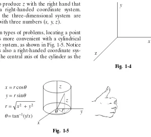
Three-dimensional coordinate systems are usually right handed. In Fig. 1-4 imagine your right hand positioned with fingers extended in the ⫹x direction
closing naturally so that your fingers rotate into the direction of the ⫹yaxis
while your thumb points in the direction of the ⫹zaxis. It is this rotation of
Fig. 1-3
Quick Tip
Be sure that you understand how to calculate q⫽tan−1(4/3) ⫽53⬚on your
cal-culator. This is not 1/tan(4/3). This is the inverse tangent. Instead of the ratio of two sides of a right triangle (the regular tangent function), the inverse tangent does the opposite: it calculates the angle from a number, the ratio of the two sides of the triangle. On most calculators you need to hit a 2ndfunction key or
”inv” key to perform this ”inverse” operation.
x y
q =tan–1(y/x)
x = r cos q
y = r sin q
x2+y2 r =
y = r sin q
xintoyto produce zwith the right hand that specifies a right-handed coordinate system. Points in the three-dimensional system are specified with three numbers (x, y, z).
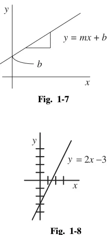
For certain types of problems, locating a point in space is more convenient with a cylindrical coordinate system, as shown in Fig. 1-5. Notice that this is also a right-handed coordinate sys-tem with the central axis of the cylinder as the
z-axis.
A point is located by specifying a radius measured out from the origin in the ⫹x
direction, an angle in the x-y plane measured from the x-axis, and a height above the x-yplane. Thus the coordinates in the cylindrical system are . The relation of these coordinates to x, y, zis given in Fig. 1-5.
1-5
Logarithms and Exponents
Logarithms and exponents are used to describe several physical phenomena. The exponential function is a unique one with the general shape shown in Fig. 1-6.
y⫽ax
(r,u,z)
Fig. 1-5
Fig. 1-6
x z
y
Fig. 1-4
x
y z
z r q = tan−1(y/x)
sinq cosq
y2
x2
r r y
r x
+ =
= =
q
x y
This exponential equation cannot be solved for xusing normal alge-braic techniques. The solution to is one of the definitions of the loga-rithmic function:
The language of exponents and logarithms is much the same. In exponential functions we say “ais the base raised to the power x.” In logarithm functions we say “xis the logarithm to the base aofy.” The laws for the manipulation of exponents and logarithms are similar. The manipulative rules for exponents and logarithms are summarized in the box below.
The term “log” is usually used to mean logarithms to the base 10, while “ln” is used to mean logarithms to the base e. The terms “natural” (for base e) and “common” (for base 10) are frequently used.
y⫽ax
1x⫽logay y⫽ ax
y⫽ ax
Example 1-9 Convert the exponential statement to a logarithmic
statement.
Solution: is the same statement as x ⫽ logay, so is 2 ⫽
log10100.
Example 1-10 Convert the exponential statement to a (natural)
log-arithmic statement.
Solution: so
Example 1-11 Convert log 2 ⫽0.301 to an exponential statement.
Solution: 100.301⫽2
ln7.4⫽2
e2⫽ 7.4
e2⫽7.4
100⫽ 102 y⫽ax
100⫽ 102
LAWS OF EXPONENTS AND LOGARITHMS
(ax)y⫽axy ylogax⫽logaxy
axay⫽ax⫹y
logax⫹logay⫽logaxy
logax⫺log
ay⫽ loga
x y ax
Example 1-12 Find log(2.1)(4.3)1.6.
Solution: On your hand calculator raise 4.3 to the 1.6 power and multiply this result by 2.1. Now take the log to obtain 1.34.
Second Solution: Applying the laws for the manipulation of logarithms write: log(2.1)(4.3)1.6⫽log 2.1 ⫹log 4.31.6⫽log 2.1 ⫹1.6 log 4.3 ⫽0.32⫹1.01⫽1.33
(Note the round-off error in this second solution.) This second solution is rarely used for numbers. It is, however, used in solving equations.
Example 1-13 Solve .
Solution: Apply a manipulative rule for logarithms: or .
Now switch to exponentials: x⫽ e3.31⫽27.4
3.31⫽ lnx
4⫽ ln2⫹lnx 4⫽ln2x
Quick Tip
A very convenient phrase to remember in working with logarithms is “a logarithm is an exponent.” If the logarithm of something is a number or an expression, then that number or expression is the exponent of the base of the logarithm.
1-6
Functions and Graphs
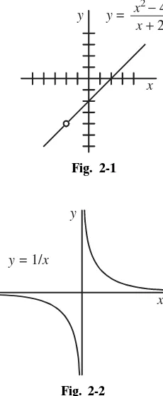
Functions can be viewed as a series of mathematical orders. The typical func-tion is written starting with y, or , read as “fofx,” short for function of x. The mathematical function is a series of orders or operations to be performed on an as yet to be specified value of x. This set of orders is: square x, add 2 times x, and add 1. The operations specified in the function can be performed on individual values of xor graphed to show a con-tinuous “function.” It is the graphing that is most encountered in calculus. We’ll look at a variety of algebraic functions eventually leading into the concept of the limit.
Example 1-14 Perform the functions on the number 2 or find .
Solution: Performing the operations on the specified function
In visualizing problems it is very helpful to know what certain functions look like. You should review the functions described in this section until you can look at a function and picture “in your mind’s eye” what it looks like. This skill will prove valuable to you as you progress through your calculus course.
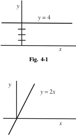
Linear
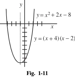
The linear algebraic function (see Fig. 1-7) is , where mis the slope of the straight line and bis the intercept, the point where the line crosses the y-axis. This is not the only form for the linear function, but it is the one that is used in graphing and is the one most easily visualized.
Example 1-15 Graph the function .
Solution: This is a straight line, and it is in the cor-rect form for graphing. Because the slope is posi-tive, the curve rises with increasing x. The coeffi-cient 2 tells you that the curve is steeper than a slope 1, (which has a 45⬚angle). The constant ⫺3 is the intercept, the point where the line crosses the y -axis. (See Fig. 1-8.)
You should go through this little visualization exer-cise with every function you graph. Knowing the general shape of the curve makes graphing much easier. With a little experience you should look at
this function and immediately visualize that (1) it is a straight line (first power), (2) it has a positive slope greater than 1 so it is a rather steep line rising to the right, and (3) the constant term means that the line crosses the y-axis at ⫺3.
Knowing generally what the line looks like, place the first (easiest) point at x⫽0,
y⫽ ⫺3. Again knowing that the line rises to the right, pick x⫽2,y⫽1, and as a check x⫽3,y⫽3.
y⫽ 2x⫺3
y⫽mx⫹ b
f(2)⫽ 23⫺3(2)⫹ 7⫽8⫺6⫹7⫽9
f(2)
f(x)⫽ x3⫺ 3x⫹7
Fig. 1-7
Fig. 1-8 y
x b
y = mx +b
x y
If you are not familiar with visualizing the function before you start calculating points, graph a few straight lines, but go through the exercise outlined above before you place any points on the graph.
Quadratics
The next most complicated function is the quadratic (see Fig. 1-9), and the simplest quadratic is , a curve of increasing slope, symmetric about the y-axis (yhas the same value for x⫽ ⫹or⫺1,⫹or⫺2, etc.). This symmetry property is very useful in graphing. Quadratics are also called parabolas. Adding a con-stant to obtain serves to move the curve up or down the y-axis in the same way the constant term moves the straight line up and down the y-axis.
Example 1-16 Graph .
Solution: First note that the curve is a parabola with the symmetry attendant to parabolas and it is moved down on the y-axis by the ⫺3. The point is the key point, being the apex or lowest point for the curve, and the defining point for the symmetry line, which is the y-axis. Now, knowing the general shape of the curve add the point . This is sufficient information to construct the graph as shown in Fig. 1-9. Further points can be added if necessary.
Adding a constant ain front of the x2either sharpens (a> 1) or flattens (a< 1)
the graph. A negative avalue causes the curve to open down.
Example 1-17 Graph .
Solution: Looking at the function, note that it is a parabola ( term), it is flatter than normal (0.5 coefficient), it opens up (positive coefficient of the term), and it is moved up the axis one unit. Now put in some numbers: is the apex, and the y-axis is the symmetry line. Add the points and sketch the graph (Fig. 1-10).
Example 1-18 Graph .
Solution: Look at the function and verify the following statement. This is a parabola that opens down, is sharper than normal, and is displaced two units in
the negative direction. Put in the two points and and verify the graph shown in Fig. 1-10.
Adding a linear term, a constant times x, so that the function has the form produces the most complicated quadratic. The addition of this constant term moves the curve both up and down and sideways. If the quadratic function is factorable then the places where it crosses the x-axis are obtained directly from the factored form.
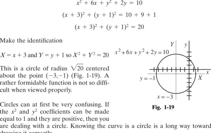
Example 1-19 Graph the function .
Solution: This is a parabola that opens up, and is displaced up or down and sideways. This quadratic is factorable to . The values and make , so these are the points where the curve crosses the
x-axis. Place these points on the graph. Now here is where the symmetry property of parabolas is used. Because of the symmetry, the parabola must be symmetric about a line halfway between and , or about the line . The apex of the parabola is on this line so substitute to find the appropriate value of y: f(⫺1) ⫽ (⫺1⫹4) (⫺1⫺2) ⫽ ⫺9. These three points are suffi-cient to sketch the curve (see Fig. 1-11).
Before moving on to the graphing of quadrat-ics that are not factorable there is one other
quadratic that is rather simple yet it illustrates the method necessary for rapid graphing of nonfactorable quadratics.
Example 1-20 Graph .
Solution: Notice in Fig. 1-12 that the right side of this equation is a perfect square and the equation can be written as . The apex of the curve is at , and any variation of xfrom⫺2 makes y positive. And the parabola is symmetric about the
line . If or , . If or
, . This is sufficient information to sketch the curve. Notice, however, in the second solu-tion an even easier means for graphing the funcsolu-tion.
Second Solution: The curve can be written in the form if is defined as . At , and the line effectively defines a new axis. Call it the Y-axis. This is the axis of symmetry determined in the previous solution. Drawing in the new axis allows graphing of the simple equation
about this new axis.
y⫽X2
Example 1-21 Graph .
Solution: Based on experience with the previous problem subtract 2 from both sides to at least get the right side a perfect square:
y⫺ 2⫽x2⫺6x⫹9⫽(x⫺ 3)2. This form of
the equation suggests the definitions and , so that the equation reads . This is a parabola of standard shape on the new coordinate sys-tem with origin at . The new coordinate axes are the lines and . This
rather formidable looking function can now be drawn quite easily with the new coordinate axes. (See Fig. 1-13.)
The key step in getting started on Example 1-21 is recognizing that subtracting 2 from both sides makes a perfect square on the right. This step is not always obvi-ous, so we need a method of converting the right-hand side into a perfect square. This method is a variation of the “completing the square” technique for solving quadratic equations. If you are not very familiar with completing the square (this should include nearly everyone) go back in this chapter and review the process before going on. Now that you have “completing the square” clearly in your mind we’ll graph a nonfactorable quadratic with a procedure that always works.
Example 1-22 Graph .
Solution: 1. Move the constant to the left side of the equation: y⫺7⫽x2⫹4x.
Next, determine what will make the right-hand side a perfect square. In this case
y⫽ x2⫹4x⫹ 7
The previous problem and the following problem illustrate the progression of perfect square to completing the square approaches to graphing quadratics. This is a valuable time-saving method of graphing.
⫹4 makes a perfect square on the right so add
this to both sides: or
.
2. Now, make the shift in axes with the
defi-nitions and . The origin
of the “new” coordinate axes is (⫺2,3). Determining the origin from these defining equations helps to prevent scrambling the (⫺2,3) and getting the origin in the wrong place. The values (⫺2,3) make X and Y zero and this is the apex of the curve on the new coordinate axes.
3. Graph the curve as shown in Fig. 1-14.
Higher Power Curves
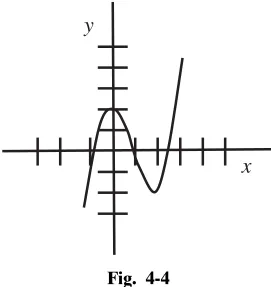
The graphing of cubic and higher power curves requires techniques you will learn in your calculus course. There are, however, some features of higher power curves that can be learned from an “algebraic” look at the curves.
The simple curves for and are shown in Fig. 1-15. Adding a constant term to either of these curves serves to move them up or down on the y-axis the same as it does for a quadratic or straight line. Cubics plus a constant are relatively easy to sketch. Adding a quadratic or linear term adds complications that are almost always easiest handled by learning the calculus necessary to help you graph the curve. If a curve contains an term, this term will eventually predominate for sufficiently large x.
Operationally, this means that if you have an expression
y⫽x3⫹()x2⫹()x⫹(), while there may be
consider-able gyration of the curve near the origin, for large
(pos-itive or negative) xthe curve will eventually take the shape shown in Fig. 1-15.
The same is true for other higher power curves. The curve is similar in shape to , it just rises more rapidly. The addition of other (lower than 4) power terms again may add some interesting twists to the curve but for large x
it will eventually rise sharply.
1-7
Conics
The next general category of curves is called conics, because they have shapes generated by passing a plane through a cone. They contain xandyterms to the second power. The simplest of these curves is generated with and equal to a constant. More complicated curves have positive coefficients for these terms, and the most complicated conics have positive and negative coefficients.
Circles
Circles are functions in the form
with the constant written in what turns out to be a convenient form, . The curve is composed of a collection of points in the x-yplane whose squares equal . Look at Fig. 1-16 and note that for each point that satisfies the equation, a right triangle can be con-structed with sides x, y, and r, and the Pythagorean theorem defines the relationship . A circle is a collection of points, equal distance from a point called the center.
Example 1-23 Graph .
Solution: Look at the function and recognize that it is a circle. It has radius 3 and it is centered about the
origin. At , , and at . Now
draw the circle (Fig. 1-17). Note that someone may try to confuse you by writing this function as . Don’t let them.
Example 1-24 Graphx2⫺6x⫹9⫹y2⫽16.
Solution: At first glance it looks as though a page is missing between Examples 1-23 and 1-24. But if you make the identifica-tion that is the perfect square
of then the equation reads
if and .
This is the identification that worked so well for parabolas. In the new coordinate system with origin at (3,0) this curve is a circle of radius 4, centered on the point (3,0) (Fig. 1-18). Set up the new coordinate system and graph
If the function were written it would not have been quite so easy to recognize the curve. Looking at this latter rearrangement, the clue that this is a circle is that the and terms are both positive when they are together on the same side of the equation. No matter how scrambled the terms are, if you can recognize that the curve is a circle you can separate out the terms and make some sense out of them by making perfect squares. This next problem will give you an example that is about as complicated as you will encounter.
Example 1-25 Graph .
Solution: Notice that the xandyterms are at least grouped together and further that the constant has been moved to the right side of the equation. This is similar to the first step in solving an equation by completing the square. Now with the equation written in this form write the perfect squares that satisfy the and x
terms and the and yterms adding the appropriate constants to the right side.
Make the identification
X⫽x⫹3 andY⫽y⫹1 soX2⫹Y2⫽20
This is a circle of radius centered about the point (⫺3,⫺1) (Fig. 1-19). A rather formidable function is not so diffi-cult when viewed properly.
Circles can at first be very confusing. If the and coefficients can be made equal to 1 and they are positive, then you
are dealing with a circle. Knowing the curve is a circle is a long way toward drawing it correctly.
Ellipses
Ellipses have and terms with positive but different coefficients. The two forms for the equation of an ellipse are
or x2
a2 ⫹ y2 b2⫽ 1 ax2⫹by2⫽c2
y2 x2 y2 x2
220
(x⫹3)2⫹ (y⫹ 1)2⫽20
(x⫹3)2⫹(y⫹ 1)2⫽10⫹ 9⫹ 1
x2⫹ 6x⫹y2⫹2y⫽10 y2
x2 x2⫹ 6x⫹y2⫹ 2y⫽10
y2 x2
y2⫽6x⫺ x2⫹ 7
Fig. 1-19 x2+6x+y +2y=10
x X y Y
x= −3 y= −1
Each form has its advantages with the latter form being the more convenient for graphing.
Example 1-26 Graph .
Solution: This is an ellipse because the xandyterms are squared and have dif-ferent positive coefficients. The difdif-ferent coefficients indicate a stretching or com-pression of the curve in the xorydirection. It is not necessary to know the direc-tion. That comes out of the graphing technique. Rewrite the equation into a more convenient form for graphing by dividing by 36.
Now in this form set first so , and then , so . With these points and the knowledge that it is a circle compressed in one direction, sketch the curve (Fig. 1-20).
Example 1-27 Graph .
Solution: The problem is presented in this somewhat artificial form to illustrate the axis shifting used so effectively in the graphing of parabolas and circles.
Based on this experience immediately write
with the definitions , Y⫽y⫺4. The origin of the new coordinate system is at (⫺1,4), and in this new coordinate
system when and when
, .
Sketch the curve (Fig. 1-21).
Example 1-28 Graphx2⫹4x⫹9y2⫺18y⫽ ⫺4.
Solution: The different positive coefficients of the and terms tell us this is an ellipse. The linear terms in xandytell us it is displaced off the x-yaxis.
Graphing this curve is going to require a completing the square approach with considerable attention to detail.
First, write .
Now do the completing the square exercise, being very careful of the 9 outside the parentheses:
Now divide to reach
Define and to achieve
Graph on the new coordinate system: when , , and when , .
Alternate Solution: An alternative to graphing in the new coordinate system is to go back to the original coordinate system. When , substitute and write
or , and when
, substitute and write
or . Either way gives the same points on the graph (Fig. 1-22).
Hyperbolas
Ellipses are different from circles because of numerical coefficients for the and terms. Hyperbolas are different from ellipses and circles because one of the coefficients of these and terms is negative. This makes the analysis somewhat more complicated. Hyperbolas are written in one of two forms, both of which are sometimes needed in the graphing.
or
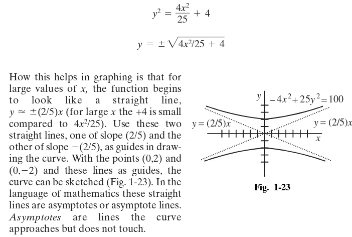
Example 1-29 Graph⫺4x2⫹25y2⫽100.
values of x. If the curve goes through the points and and does not exist along the line , then the curve must have two separate parts! Rearrange the equation to and note immediately that for real values of x,yhas to be greater than 2 or less than ⫺2. The curve does not exist in the region bounded by the lines and .
At this point in the analysis we have two points and a region where the curve does not exist. Further analysis requires a departure from the usual techniques applied to conics. Rewrite the equation again, but this time in the form y⫽…
How this helps in graphing is that for large values of x, the function begins to look like a straight line, (for large xthe +4 is small compared to ). Use these two straight lines, one of slope and the other of slope ⫺(2/5), as guides in draw-ing the curve. With the points and and these lines as guides, the curve can be sketched (Fig. 1-23). In the language of mathematics these straight lines are asymptotes or asymptote lines.
Asymptotes are lines the curve approaches but does not touch.
Now that you know the general shape of hyperbolas, we can look at some hyperbolas that are not symmetric about the origin. The next problem is some-what artificial, but it is instructive and illustrates a situation that comes up in the graphing of hyperbolas.
Example 1-30 Graph .
Solution: This function is in a convenient form for graphing, especially if we make the identification and . This hyperbola is displaced up and down and sideways to the new coordinate system with origin at (1,3). In
this new coordinate system at , Ydoes not have any real values. At Y⫽0, . Place these points on the graph.
The asymptote lines are most easily drawn in the new coordinate system.
The transformed function is
and for large values of X,
9Y2⫽4X2⫺36
Straight lines of slope ⫹(2/3) and ⫺(2/3) are drawn in the new coordinate sys-tem. With the two points and these asymptote lines the curve can be sketched. In Fig. 1-24 you will see a rectangle. This
is used by some as a convenient con-struct for drawing the asymptote lines and finding the critical points of the curve. Two sides of the rectangle inter-sect the X-axis at the points where the curve crosses this axis and the diagonals of the rectangle have slopes .
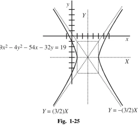
Example 1-31 Graph 9x2⫺4y2⫺54x
⫺32y⫽19.
Solution: This is a hyperbola, and the presence of the linear terms indicates it is moved up and down and sideways. Graphing requires a completing the square approach. Follow the completing the square approach through the equa-tions below. Watch the multiplication of the parentheses very carefully.
Make the identification and so the function can be written
or X2 4 ⫺
Y2
9 ⫽1 9X2⫺4Y2⫽36
Y⫽y⫹4
X⫽x⫺3
9(x⫺3)2⫺ 4(y⫹4)2⫽ 19⫹81⫺ 64⫽36 9(x2⫺ 6x)⫺ 4(y2⫹8y)⫽19
9x2⫺4y2⫺54x⫺32y⫽19
⫾(2/3)
Y<⫾(2/3)X
Y<⫾(2/3)X
Y2⫽ (4/9)X2⫺ 4
X2
9 ⫺
Y2
4 ⫽1 (x⫺1)2
9 ⫺
(y⫺3)2
4 ⫽ 1
X⫽ ⫾3
X⫽0
Fig. 1-24 x y
Draw in the new axes with origin at . When X⫽ 0, there are no real Y values. When , . Place these points on the graph. The asymptotes come out of the y⫽ … equation. Follow along the rearrangement to find the asymptote lines. (See Fig. 1-25.)
For large values of X, . The addition of these asymptote lines allows completion of the graph.
Y<⫾(3/2)X
Y⫽ ⫾2(9/4)X2⫺9
Y2⫽ (9/4)X2⫺9 X⫽ ⫾2
Y⫽0
(3,⫺4)
Quick Tip
In graphing conics the first thing to determine is whether the equation is a cir-cle, ellipse, or hyperbola. This is accomplished by looking at the numerical coef-ficients, their algebraic signs, and whether they are (numerically) different. Knowing the curve, the analytical techniques begin by looking for the values of x when y ⫽0, and the values of y when x ⫽0. The answers to these questions
give the intercepts for the circle and ellipse, and the square root of a negative number for one determines that the curve is a hyperbola. The addition of linear terms moves the conics up and down and sideways and almost always requires a completing the square type of analysis, complete with axis shifting.
Fig. 1-25
x y
X Y
Y = (3/2)X Y = −(3/2)X
If you can figure out what the curve looks like and can find the intercepts ( and ) you are a long way toward graphing the function. The shifting of axes just takes attention to detail.
1-8
Graphing Trigonometric Functions
Graphing the trigonometric functions does not usually present any prob-lems. There are a few pitfalls, but with the correct graphing technique these can be avoided. Before graphing the functions you need to know their gen-eral shape. The trigonometric relations are defined in an earlier section and their functions shown graphically. If you are not very familiar with the shape of the sine, cosine, and tangent functions draw them out on a 3 ⫻5 card and use this card as a bookmark in your text or study guide and review it every time you open your book (possibly even more often) until the word sine projects an image of a sine function in your mind, and likewise for cosine and tangent.
Let’s look first at the sine function
and its graph in Fig. 1-26. The , called the argument of the function, is cyclic in ; when-ever goes from 0 to the sine function goes through one cycle. Also notice that there is a symmetry in the function. The shape of the curve from 0 to is mirrored in the shape from to . Similarly, the shape of the curve from 0 to is mirrored in the shape from to . In order to draw the complete sine curve
we only need to know the points defining the first quarter cycle. This property of sine curves that allows construction of the entire curve if the points for the first quarter cycle are known will prove very
valu-able in graphing sine functions with complex arguments. Operationally, the values of the function are determined by “punching them up” on a hand calculator.
Example 1-32 Graph .
Solution: The 2 here is called the amplitude
and simply scales the curve in the ydirection. It is handled simply by labeling the y-axis, as shown in Fig. 1-27.
Example 1-33 Graph .
Solution: The phrase “cos” describes the general shape of the curve, the unique cosine shape. The is the hard part. Look back at the basic shape of the cosine curve and note that when , the cosine curve has gone through of its cycle. The values of xfor the points where 2xis zero and define the first quarter cycle. (One-quarter of a cycle is all that is necessary to graph the function.) To graph this function (yvs.x) we need to know only those values ofxwhere the argument of the function ( ) is zero and . The chart in Fig. 1-28 shows the values necessary for graphing the function.
p/2
Do not start this chart with values of x; start with values for 2x. Read the previ-ous sentence again. It is the key to correctly graphing trigonometric functions. Notice that the points on the x-axis are written as multiples of the first quarter cycle. It is a cumbersome way of writing the points, but it helps prevent mistakes in labeling the x-axis.
Go back over the logic of graphing trigonometric functions in this way. It is the key to always getting them graphed correctly. As the functions become more complicated, the utility and logic of this approach will become more evident.
Example 1-34 Graph .
Solution: This is a sine function: the gener-al shape of which can be seen clearly in your
mind’s eye. The amplitude of 2 is no problem. The argument requires setting up a chart to find the values of xdefining the first quarter cycle of the sine func-tion. Numbers associated with the argument of the function, the 3 (in the denom-inator) in this case, define the frequencyof the function. While interesting in some contexts, knowing the frequency is not important in graphing. (Discussion of the frequency of periodic functions is contained in Physics for the Utterly Confused.)
Remember, in setting up the chart set equal to zero and solve for x. The sine of zero is zero. Next set equal to and solve for x. The sine of is 1. These two points define the first quarter cycle of the function. The remainder of the function is drawn in (Fig. 1-29) using the symmetry properties of sine functions.
Example 1-35 Graph .
Solution: The introduction of the pin the argument of the function is the final complication in graphing trigonometric functions. This con-stant in the argument is called the
phaseand the sign of this constant
moves the function to the left or right on the
x-axis. It is not necessary to remember which sign moves the function which way. The place-ment of the function on the x-axis comes out of the analysis.
Figure 1-30 shows a sine function with ampli-tude 1. The 2 affects the frequency and the moves the function right or left. Set up the p chart again forcing the argument to be zero or and determining the appropriate xvalue.
Set and solve for .
Set and solve for . Draw the graph starting with the first quarter cycle of the sine function in the region from to .
Example 1-36 Graph .
Solution: The function shown in Fig. 1-31 has another little twist to it, which has to do with the minus sign.
Follow the development of the chart and take 2x⫺p/3⫽ 0 for the first point. This
Set up the x-ycoordinate system and place the first quarter of the cosine function between and . With this section of the cosine function complete, draw in the remainder of the curve.
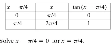
Example 1-37 Graph .
Solution: If you are at all unfamiliar with the tangent function go back and review it in the trigonometry section. The important features as far as graphing is concerned are that is zero when is zero and is 1 when is . The tangent curve goes infi-nite when goes to , but a point at infin-ity is not an easy one to deal with.
For the function shown in Fig. 1-32, set up a chart and find the values of x that make equal zero and . These two points allow construction of the function.
p/4
Be careful while graphing the tangent function, especially this one. This tangent function is zero when , and 1 when . The standard mistake is to take the function to infinity at .
✔
Solve quadratic equations either by factoring or formula✔
Keep the image of the sine, cosine, and tangent functions in your mind✔
Graph trigonometric functions using the advanced techniques✔
Switch from rectangular to polar coordinate systems and vice versa✔
Know the basic laws for manipulating logarithms and exponents✔
Evaluate and graph functions✔
Graph circles (equal and positive coefficients of the x2andy2terms)✔
Graph ellipses (nonequal and positive coefficients of the x2andy2terms)✔
Graph hyperbolas (nonequal and one “⫺” sign of the x2andy2terms)PROBLEMS
1. Solve by factoring .
2. Solve by factoring .
3. Solve by quadratic formula . 4. Solve by quadratic formula . 5. Write using the binomial expansion. 6. Convert p/4 rad to degrees.
7. Convert 0.45 rad to degrees. 8. Convert 2.6 rad to degrees. 9. Convert 80⬚to radians. 10. Convert 200⬚to radians.
11. Switch the point (⫺4,6) to polar form. 12. Switch the point (2,⫺5) to polar form. 13. Switch 3 @ 20⬚to rectangular form. 14. Switch 5 @ 60⬚to rectangular form. 15. Solve 6 ⫽ln3xforx.
16. Solve . 17. Solve .
18. Write log3 = 0.48 in exponential form. 19. Solve .
20. Evaluate log(3.6)(4.1)3.
21. Evaluate log[(4.2)2/2.3].
ANSWERS
11. This problem requires a diagram. There are two problems: first remember that the angle has to be measured counter-clockwise from the positive
x-axis, and second be careful how you measure the angle. The angle measured from the ⫺x axis is determined by tan⫺1(6/4) ⫽ 56.3⬚. Now subtract
56.3⬚from 180⬚for 123.7⬚. This is the correct num-ber for the angle. The magnitude is the square root of 6 squared plus 4 squared or square root of . Written in polar form the coordinates are 7.2 @ 123.7⬚.
12. This problem requires a diagram. There are two problems: first remember that the angle has to be measured counterclockwise from the positive x-axis, and second be careful how you measure the angle. If you try and take the inverse tangent of 2 divided by ⫺5, you will get a negative number—very confusing. The safest way to do this problem is to find the small angle between the y-axis and the arrow. Take the