John von Neumann Institute for Computing
Ab initio molecular dynamics: Theory and
Implementation
Dominik Marx and J ¨urg Hutter
published in
Modern Methods and Algorithms of Quantum Chemistry,
J. Grotendorst (Ed.), John von Neumann Institute for Computing,
J ¨ulich, NIC Series, Vol.
1
, ISBN 3-00-005618-1, pp. 301-449, 2000.
c
2000 by John von Neumann Institute for Computing
Permission to make digital or hard copies of portions of this work for personal or classroom use is granted provided that the copies are not made or distributed for profit or commercial advantage and that copies bear this notice and the full citation on the first page. To copy otherwise requires prior specific permission by the publisher mentioned above.
AB INITIOMOLECULAR DYNAMICS: THEORY AND IMPLEMENTATION
DOMINIK MARX
Lehrstuhl f¨ur Theoretische Chemie, Ruhr–Universit¨at Bochum Universit¨atsstrasse 150, 44780 Bochum, Germany E–mail: [email protected]
J ¨URG HUTTER
Organisch–chemisches Institut, Universit¨at Z¨urich Winterthurerstrasse 190, 8057 Z¨urich, Switzerland
E–mail: [email protected]
The rapidly growing field ofab initiomolecular dynamics is reviewed in the spirit of a series of lectures given at the Winterschool 2000 at theJohn von Neumann Institute for Computing, J¨ulich. Several such molecular dynamics schemes are compared which arise from following various approximations to the fully coupled Schr¨odinger equation for electrons and nuclei. Special focus is given to the Car– Parrinello method with discussion of both strengths and weaknesses in addition to its range of applicability. To shed light upon why the Car–Parrinello approach works several alternate perspectives of the underlying ideas are presented. The implementation of ab initio molecular dynamics within the framework of plane wave–pseudopotential density functional theory is given in detail, including diag-onalization and minimization techniques as required for the Born–Oppenheimer variant. Efficient algorithms for the most important computational kernel routines are presented. The adaptation of these routines to distributed memory parallel computers is discussed using the implementation within the computer codeCPMD as an example. Several advanced techniques from the field of molecular dynam-ics, (constant temperature dynamdynam-ics, constant pressure dynamics) and electronic structure theory (free energy functional, excited states) are introduced. The com-bination of the path integral method withab initiomolecular dynamics is presented in detail, showing its limitations and possible extensions. Finally, a wide range of applications from materials science to biochemistry is listed, which shows the enor-mous potential ofab initiomolecular dynamics for both explaining and predicting properties of molecules and materials on an atomic scale.
1 Setting the Stage: Why Ab InitioMolecular Dynamics ?
Classical molecular dynamics using “predefined potentials”, either based on em-pirical data or on independent electronic structure calculations, is well estab-lished as a powerful tool to investigate many–body condensed matter systems. The broadness, diversity, and level of sophistication of this technique is docu-mented in several monographs as well as proceedings of conferences and scientific schools 12,135,270,217,69,59,177. At the very heart of any molecular dynamics scheme
is the question of how to describe – that is in practice how to approximate – the interatomic interactions. The traditional route followed in molecular dynamics is to determine these potentials in advance. Typically, the full interaction is broken up into two–body, three–body and many–body contributions, long–range and short– range terms etc., which have to be represented by suitable functional forms, see Sect. 2 of Ref. 253 for a detailed account. After decades of intense research, very
analytically were devised253,539,584.
Despite overwhelming success – which will however not be praised in this re-view – the need to devise a “fixed model potential” implies serious drawbacks, see the introduction sections of several earlier reviews 513,472for a more complete
di-gression on these aspects. Among the most delicate ones are systems where (i) many different atom or molecule types give rise to a myriad of different interatomic interactions that have to be parameterized and / or (ii) the electronic structure and thus the bonding pattern changes qualitatively in the course of the simulation. These systems can be called “chemically complex”.
The reign of traditional molecular dynamicsand electronic structure methods was greatly extended by the family of techniques that is called here “ab initio
molecular dynamics”. Other names that are currently in use are for instance Car– Parrinello, Hellmann–Feynman, first principles, quantum chemical, on–the–fly, di-rect, potential–free, quantum, etc. molecular dynamics. The basic idea underlying every ab initiomolecular dynamics method is to compute the forces acting on the nuclei from electronic structure calculations that are performed “on–the–fly” as the molecular dynamics trajectory is generated. In this way, the electronic variables are not integrated out beforehand, but are considered as active degrees of freedom. This implies that, given a suitable approximate solution of the many–electron problem, also “chemically complex” systems can be handled by molecular dynamics. But this also implies that the approximation is shifted from the level of selecting the model potential to the level of selecting a particular approximation for solving the Schr¨odinger equation.
Applications ofab initiomolecular dynamics are particularly widespread in ma-terials science and chemistry, where the aforementioned difficulties (i) and (ii) are particularly severe. A collection of problems that were already tackled byab initio
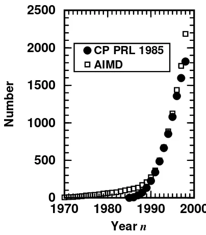
molecular dynamics including the pertinent references can be found in Sect. 5. The power of this novel technique lead to an explosion of the activity in this field in terms of the number of published papers. The locus can be located in the late–eighties, see the squares in Fig. 1 that can be interpreted as a measure of the activity in the area ofab initiomolecular dynamics. As a matter of fact the time evolution of the number of citations of a particular paper, the one by Car and Parrinello from 1985 entitled “Unified Approach for Molecular Dynamics and Density–Functional Theory” 108, parallels the trend in the entire field, see the circles in Fig. 1. Thus,
the resonance that the Car and Parrinello paper evoked and the popularity of the entire field go hand in hand in the last decade. Incidentally, the 1985 paper by Car and Parrinello is the last one included in the section “Trends and Prospects” in the reprint collection of “key papers” from the field of atomistic computer simula-tions135. That the entire field ofab initiomolecular dynamics has grown mature
is also evidenced by a separate PACS classification number (71.15.Pd “Electronic Structure: Molecular dynamics calculations (Car–Parrinello) and other numerical simulations”) that was introduced in 1996 into the Physics and Astronomy Classi-fication Scheme 486.
1970
1980
1990
2000
Year
n
0
500
1000
1500
2000
2500
Number
CP PRL 1985 AIMD
Figure 1. Publication and citation analysis. Squares: number of publications which appeared up to the yearnthat contain the keyword “ab initiomolecular dynamics” (or synonyma such as “first principles MD”, “Car–Parrinello simulations” etc.) in title, abstract or keyword list. Circles: number of publications which appeared up to the yearn that cite the 1985 paper by Car and Parrinello108
(including misspellings of the bibliographic reference). Self–citations and self–papers are excluded, i.e. citations of Ref.108
in their own papers and papers coauthored by R. Car and / or M. Parrinello arenotconsidered in the respective statistics. The analysis is based on the CAPLUS (“Chemical Abstracts Plus”), INSPEC (“Physics Abstracts”), and SCI (“Science Citation Index”) data bases at STN International. Updated statistics from Ref.405
.
standard molecular dynamics. Another appealing feature of standard molecular dynamics is less evident, namely the “experimental aspect of playing with the po-tential”. Thus, tracing back the properties of a given system to a simple physical picture or mechanism is much harder in ab initiomolecular dynamics. The bright side is that new phenomena, which were not forseen before starting the simulation, can simply happen if necessary. This gives ab initio molecular dynamics a truly predictive power.
Ab initiomolecular dynamics can also be viewed from another corner, namely from the field of classical trajectory calculations 649,541. In this approach, which
the first one, why so? There are 3N−6 internal degrees of freedom that span the global potential energy surface of an unconstrainedN–body system. Using for sim-plicity 10 discretization points per coordinate implies that of the order of 103N−6
electronic structure calculations are needed in order to map such a global potential energy surface. Thus, the computational workload for the first step grows roughly like∼10N with increasing system size. This is what might be called the “dimen-sionality bottleneck” of calculations that rely on globalpotential energy surfaces, see for instance the discussion on p. 420 in Ref. 254.
What is needed inab initiomolecular dynamics instead? Suppose that a useful trajectory consists of about 10M molecular dynamics steps, i.e. 10M electronic structure calculations are needed to generate one trajectory. Furthermore, it is assumed that 10n independent trajectories are necessary in order to average over different initial conditions so that 10M+n ab initiomolecular dynamics steps are required in total. Finally, it is assumed that each single–point electronic structure calculation needed to devise the global potential energy surface and one ab initio
molecular dynamics time step requires roughly the same amount ofcputime. Based on this truly simplistic order of magnitude estimate, the advantage of ab initio
molecular dynamics vs. calculations relying on the computation of a global potential energy surface amounts to about 103N−6−M−n. The crucial point is that for a given statistical accuracy (that is for M andn fixed and independent onN) and for a given electronic structure method, the computational advantage of “on–the–fly” approaches grows like ∼10N with system size.
Of course, considerable progress has been achieved in trajectory calculations by carefully selecting the discretization points and reducing their number, choosing so-phisticated representations and internal coordinates, exploiting symmetry etc. but basically the scaling ∼10N with the number of nuclei remains a problem. Other strategies consist for instance in reducing the number of active degrees of freedom by constraining certain internal coordinates, representing less important ones by a (harmonic) bath or friction, or building up the global potential energy surface in terms of few–body fragments. All these approaches, however, invoke approxima-tions beyond the ones of the electronic structure method itself. Finally, it is evident that the computational advantage of the “on–the–fly” approaches diminish as more and more trajectories are needed for a given (small) system. For instance extensive averaging over many different initial conditions is required in order to calculate quantitatively scattering or reactive cross sections. Summarizing this discussion, it can be concluded that ab initio molecular dynamics is the method of choice to investigate large and “chemically complex” systems.
Quite a few review articles dealing withab initiomolecular dynamics appeared in the nineties 513,223,472,457,224,158,643,234,463,538,405and the interested reader is
but all three ab initioapproaches to molecular dynamics are contrasted and partly compared. The important issue of how to obtain the correct forces in these schemes is discussed in some depth. The most popular electronic structure theories imple-mented withinab initiomolecular dynamics, density functional theory in the first place but also the Hartree–Fock approach, are sketched. Some attention is also given to another important ingredient in ab initiomolecular dynamics, the choice of the basis set.
Concerning the depth, the focus of the present discussion is clearly the im-plementation of both the basic Car–Parrinello and Born–Oppenheimer molecular dynamics schemes in the CPMD package 142. The electronic structure approach
in CPMDis Hohenberg–Kohn–Sham density functional theory within a plane wave / pseudopotential implementation and the Generalized Gradient Approximation. The formulae for energies, forces, stress, pseudopotentials, boundary conditions, optimization procedures, parallelization etc. are given for this particular choice to solve the electronic structure problem. One should, however, keep in mind that a variety of other powerful ab initio molecular dynamics codes are available (for instance CASTEP 116, CP-PAW 143, fhi98md 189, NWChem 446, VASP 663) which are partly based on very similar techniques. The classic Car–Parrinello approach 108
is then extended to other ensembles than the microcanonical one, other electronic states than the ground state, and to a fully quantum–mechanical representation of the nuclei. Finally, the wealth of problems that can be addressed using ab initio
molecular dynamics is briefly sketched at the end, which also serves implicitly as the “Summary and Conclusions” section.
2 Basic Techniques: Theory
2.1 Deriving Classical Molecular Dynamics
The starting point of the following discussion is non–relativistic quantum mechanics as formalized via the time–dependent Schr¨odinger equation
i ∂
∂tΦ({ri},{RI};t) =HΦ({ri},{RI};t) (1)
in its position representation in conjunction with the standard Hamiltonian
H=−X
The goal of this section is to derive classical molecular dynamics 12,270,217
starting from Schr¨odinger’s wave equation and following the elegant route of Tully 650,651. To this end, the nuclear and electronic contributions to the total
wavefunction Φ({ri},{RI};t), which depends on both the nuclear and electronic coordinates, haveto be separated. The simplest possible form is a product ansatz
Φ({ri},{RI};t)≈Ψ({ri};t)χ({RI};t) exp
where the nuclear and electronic wavefunctions are separately normalized to unity at every instant of time, i.e. hχ;t|χ;ti = 1 and hΨ;t|Ψ;ti = 1, respectively. In addition, a convenient phase factor
˜
Ee= Z
drdR Ψ⋆({ri};t)χ⋆({RI};t)HeΨ({ri};t)χ({RI};t) (4) was introduced at this stage such that the final equations will look nice; RdrdR
refers to the integration over alli= 1, . . . andI= 1, . . . variables{ri}and {RI}, respectively. It is mentioned in passing that this approximation is called a one– determinant or single–configuration ansatz for thetotalwavefunction, which at the end must lead to a mean–field description of the coupled dynamics. Note also that this product ansatz (excluding the phase factor) differs from the Born–Oppenheimer ansatz340,350for separating the fast and slow variables
ΦBO({ri},{RI};t) =
even in its one–determinant limit, where only a single electronic statek(evaluated for the nuclear configuration{RI}) is included in the expansion.
Inserting the separation ansatz Eq. (3) into Eqs. (1)–(2) yields (after multiplying from the left by hΨ| andhχ|and imposing energy conservation dhHi/dt≡0) the
This set of coupled equations defines the basis of the time–dependent self–consistent field (TDSCF) method introduced as early as 1930 by Dirac162, see also Ref. 158.
The next step in the derivation of classical molecular dynamics is the task to approximate the nuclei as classical point particles. How can this be achieved in the framework of the TDSCF approach, given one quantum–mechanical wave equa-tion describing all nuclei? A well–known route to extract classical mechanics from quantum mechanics in general starts with rewriting the corresponding wavefunction
χ({RI};t) =A({RI};t) exp [iS({RI};t)/ ] (8) in terms of an amplitude factor Aand a phaseS which are both considered to be real and A >0 in this polar representation, see for instance Refs.163,425,535. After
transforming the nuclear wavefunction in Eq. (7) accordingly and after separating the real and imaginary parts, the TDSCF equation for the nuclei
∂S
is (exactly) re–expressed in terms of the new variables A and S. This so–called “quantum fluid dynamical representation” Eqs. (9)–(10) can actually be used to solve the time–dependent Schr¨odinger equation 160. The relation forA, Eq. (10),
can be rewritten as a continuity equation 163,425,535 with the help of the
identi-fication of the nuclear density |χ|2 ≡ A2 as directly obtained from the definition
Eq. (8). This continuity equation is independent of and ensures locally the con-servation of the particle probability|χ|2associated to the nuclei in the presence of
a flux.
More important for the present purpose is a more detailed discussion of the relation for S, Eq. (9). This equation contains one term that depends on , a contribution that vanishes if the classical limit
∂S
is taken as →0; an expansion in terms of would lead to a hierarchy of semi-classical methods425,259. The resulting equation is now isomorphic to equations of
motion in the Hamilton–Jacobi formulation244,540
∂S
∂t +H({RI},{∇IS}) = 0 (12)
of classical mechanics with the classical Hamilton function
H({RI},{PI}) =T({PI}) +V({RI}) (13) defined in terms of (generalized) coordinates {RI} and their conjugate momenta
{PI}. With the help of the connecting transformation
the Newtonian equation of motionP˙I =−∇IV({RI}) corresponding to Eq. (11)
dPI
dt =−∇I
Z
drΨ⋆HeΨ or
MIR¨I(t) =−∇I
Z
drΨ⋆HeΨ (15)
=−∇IVeE({RI(t)}) (16) can be read off. Thus, the nuclei move according to classical mechanics in an effective potentialVE
e due to the electrons. This potential is a function of only the
nuclear positions at time tas a result of averagingHe over the electronic degrees
of freedom, i.e. computing its quantum expectation valuehΨ|He|Ψi, while keeping
the nuclear positions fixed at their instantaneous values{RI(t)}.
However, the nuclear wavefunction still occurs in the TDSCF equation for the electronic degrees of freedom and has to be replaced by the positions of the nuclei for consistency. In this case the classical reduction can be achieved simply by replacing the nuclear density|χ({RI};t)|2in Eq. (6) in the limit →0 by a product of delta functionsQIδ(RI−RI(t)) centered at the instantaneous positions{RI(t)}of the classical nuclei as given by Eq. (15). This yields e.g. for the position operator
Z
dRχ⋆({RI};t)RI χ({RI};t)
✁
→0
−→ RI(t) (17) the required expectation value. This classical limit leads to a time–dependent wave equation for the electrons
i ∂Ψ ∂t =−
X
i 2
2me∇ 2
iΨ +Vn−e({ri},{RI(t)})Ψ
=He({ri},{RI(t)}) Ψ({ri},{RI};t) (18) which evolve self–consistently as the classical nuclei are propagated via Eq. (15). Note that nowHe and thus Ψ dependparametricallyon the classical nuclear posi-tions {RI(t)} at time t through Vn−e({ri},{RI(t)}). This means that feedback between the classical and quantum degrees of freedom is incorporated in both directions (at variance with the “classical path” or Mott non–SCF approach to dynamics 650,651).
The approach relying on solving Eq. (15) together with Eq. (18) is sometimes called “Ehrenfest molecular dynamics” in honor of Ehrenfest who was the first to address the question aof how Newtonian classical dynamics can be derived from Schr¨odinger’s wave equation 174. In the present case this leads to a hybrid or
mixed approach because only the nuclei are forced to behave like classical particles, whereas the electrons are still treated as quantum objects.
Although the TDSCF approach underlying Ehrenfest molecular dynamics clearly is a mean–field theory, transitions between electronic states are included
aThe opening statement of Ehrenfest’s famous 1927 paper174
reads:
in this scheme. This can be made evident by expanding the electronic wavefunc-tion Ψ (as opposed to the totalwavefunction Φ according to Eq. (5)) in terms of many electronic states or determinants Ψk
Ψ({ri},{RI};t) =
∞
X
k=0
ck(t)Ψk({ri};{RI}) (19)
with complex coefficients {ck(t)}. In this case, the coefficients {|ck(t)|2} (with
P
k|ck(t)|2≡1) describe explicitly the time evolution of the populations (occupa-tions) of the different states{k}whereas interferences are included via the{c⋆
kcl6=k} contributions. One possible choice for the basis functions{Ψk}is the adiabatic basis obtained from solving the time–independent electronic Schr¨odinger equation
He({ri};{RI})Ψk =Ek({RI})Ψk({ri};{RI}) , (20) where{RI}are the instantaneous nuclear positions at timetaccording to Eq. (15). The actual equations of motion in terms of the expansion coefficients {ck} are presented in Sect. 2.2.
At this stage a further simplification can be invoked by restricting the total electronic wave function Ψ to be the ground state wave function Ψ0of He at each
instant of time according to Eq. (20) and|c0(t)|2≡1 in Eq. (19). This should be a
good approximation if the energy difference between Ψ0and the first excited state
Ψ1is everywhere large compared to the thermal energykBT, roughly speaking. In
this limit the nuclei move according to Eq. (15) on a single potential energy surface
VeE= Z
drΨ⋆0HeΨ0≡E0({RI}) (21) that can be computed by solving thetime–independentelectronic Schr¨odinger equa-tion Eq. (20)
HeΨ0=E0Ψ0 , (22)
for the ground state only. This leads to the identification VE
e ≡E0 via Eq. (21),
i.e. in this limit the Ehrenfest potential is identical to the ground–state Born– Oppenheimer potential.
As a consequence of this observation, it is conceivable to decouple the task of generating the nuclear dynamics from the task of computing the potential energy surface. In a first step E0 is computed for many nuclear configurations by solving
Eq. (22). In a second step, these data points are fitted to an analytical functional form to yield a global potential energy surface 539, from which the gradients can be
obtained analytically. In a third step, the Newtonian equation of motion Eq. (16) is solved on this surface for many different initial conditions, producing a “swarm” of classical trajectories. This is, in a nutshell, the basis of classical trajectory cal-culationson global potential energy surfaces 649,541.
global potential energy surface
VE
e ≈Veapprox({RI}) =
N
X
I=1
v1(RI) + N
X
I<J
v2(RI,RJ)
+ N
X
I<J<K
v3(RI,RJ,RK) +· · · (23)
in terms of a truncated expansion of many–body contributions 253,12,270. At this
stage, the electronic degrees of freedom are replaced by interaction potentials{vn} and are not featured as explicit degrees of freedom in the equations of motion. Thus, the mixed quantum / classical problem is reduced to purely classical mechanics, once the{vn}are determined. Classical molecular dynamics
MIR¨I(t) =−∇IVeapprox({RI(t)}) (24)
relies crucially on this idea, where typically only two–body v2 or three–body v3
interactions are taken into account 12,270, although more sophisticated models to
include non–additive interactions such as polarization exist. This amounts to a dramatic simplification and removes the dimensionality bottleneck as the global potential surface is constructed from a manageable sum of additive few–body con-tributions — at the price of introducing a drastic approximation and of basically excluding chemical transformations from the realm of simulations.
As a result of this derivation, the essential assumptions underlying classical molecular dynamics become transparent: the electrons follow adiabatically the clas-sical nuclear motion and can be integrated out so that the nuclei evolve on a single Born–Oppenheimer potential energy surface (typically but not necessarily given by the electronic ground state), which is in general approximated in terms of few–body interactions.
Actually, classical molecular dynamics for many–body systems is only made possible by somehow decomposing the global potential energy. In order to illustrate this point consider the simulation ofN = 500 Argon atoms in the liquid phase 175 where the interactions can faithfully be described by additive two–body terms,
i.e. Vapprox
e ({RI}) ≈PNI<Jv2(|RI−RJ|). Thus, the determination of the pair potentialv2from ab initioelectronic structure calculations amounts to computing
and fitting a one–dimensional function. The corresponding task to determine a global potential energy surface amounts to doing that in about 101500 dimensions,
which is simply impossible (and on top of that not necessary for Nobel gases!).
2.2 Ehrenfest Molecular Dynamics
solv-ing numerically
MIR¨I(t) =−∇I
Z
drΨ⋆H
eΨ
=−∇IhΨ|He|Ψi (25)
=−∇IhHei
=−∇IVeE
i ∂Ψ ∂t =
"
−X
i 2
2me∇ 2
i +Vn−e({ri},{RI(t)})
#
Ψ
=HeΨ (26)
the coupled set of equations simultaneously. Thereby, the a priori construction of any type of potential energy surface is avoided from the outset by solving the time–dependent electronic Schr¨odinger equation “on–the–fly”. This allows one to compute the force from∇IhHeifor each configuration{RI(t)}generated by molec-ular dynamics; see Sect. 2.5 for the issue of using the so–called “Hellmann–Feynman forces” instead.
The corresponding equations of motion in terms of the adiabatic basis Eq. (20) and the time–dependent expansion coefficients Eq. (19) read 650,651
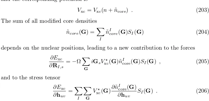
MIR¨I(t) =−
X
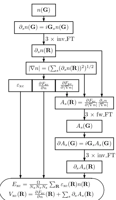
k
|ck(t)|2∇IEk−
X
k,l
c⋆kcl(Ek−El)dklI (27)
i c˙k(t) =ck(t)Ek−i
X
I,l
cl(t)R˙IdklI , (28)
where the coupling terms are given by
dklI ({RI(t)}) =
Z
drΨ⋆k∇IΨl (29) with the property dkk
I ≡0. The Ehrenfest approach is thus seen to include rigor-ously non–adiabatic transitions between different electronic states Ψkand Ψlwithin the framework of classical nuclear motion and the mean–field (TDSCF) approxi-mation to the electronic structure, see e.g. Refs.650,651for reviews and for instance
Ref. 532for an implementation in terms of time–dependent density functional
the-ory.
The restriction to one electronic state in the expansion Eq. (19), which is in most cases the ground state Ψ0, leads to
MIR¨I(t) =−∇IhΨ0|He|Ψ0i (30)
i ∂Ψ0
∂t =HeΨ0 (31)
as a special case of Eqs. (25)–(26); note thatHe is time–dependent via the nuclear
Ehrenfest molecular dynamics is certainly the oldest approach to “on–the–fly” molecular dynamics and is typically used for collision– and scattering–type prob-lems154,649,426,532. However, it was never in widespread use for systems with many
active degrees of freedom typical for condensed matter problems for reasons that will be outlined in Sec. 2.6 (although a few exceptions exist 553,34,203,617but here
the number of explicitly treated electrons is fairly limited with the exception of Ref. 617).
2.3 Born–Oppenheimer Molecular Dynamics
An alternative approach to include the electronic structure in molecular dynamics simulations consists in straightforwardly solving thestaticelectronic structure prob-lem in each molecular dynamics step given the set offixednuclear positions at that instance of time. Thus, the electronic structure part is reduced to solving atime– independent quantum problem, e.g. by solving the time–independent Schr¨odinger equation, concurrently to propagating the nuclei via classical molecular dynamics. Thus, the time–dependence of the electronic structure is a consequence of nuclear motion, and not intrinsic as in Ehrenfest molecular dynamics. The resulting Born– Oppenheimer molecular dynamics method is defined by
MIR¨I(t) =−∇Imin
Ψ0 {h
Ψ0|He|Ψ0i} (32)
E0Ψ0 =HeΨ0 (33)
for the electronic ground state. A deep difference with respect to Ehrenfest dy-namics concerning the nuclear equation of motion is that the minimum of hHei
has to be reached in each Born–Oppenheimer molecular dynamics step according to Eq. (32). In Ehrenfest dynamics, on the other hand, a wavefunction that min-imized hHei initially will also stay in its respective minimum as the nuclei move
according to Eq. (30)!
A natural and straightforward extension281of ground–state Born–Oppenheimer
dynamics is to apply the same scheme to any excited electronic state Ψk without considering any interferences. In particular, this means that also the “diagonal correction terms”340
DIkk({RI(t)}) =−
Z
drΨ⋆k∇2IΨk (34) are always neglected; the inclusion of such terms is discussed for instance in Refs. 650,651. These terms renormalize the Born–Oppenheimer or “clamped
nu-clei” potential energy surface Ek of a given state Ψk (which might also be the ground state Ψ0) and lead to the so–called “adiabatic potential energy surface”
of that state 340. Whence, Born–Oppenheimer molecular dynamics should not be
called “adiabatic molecular dynamics”, as is sometime done.
It is useful for the sake of later reference to formulate the Born–Oppenheimer equations of motion for the special case of effective one–particle Hamiltonians. This might be the Hartree–Fock approximation defined to be the variational minimum of the energy expectation valuehΨ0|He|Ψ0igiven a single Slater determinant Ψ0=
hψi|ψji=δij. The corresponding constraint minimization of the total energy with
can be cast into Lagrange’s formalism
L=− hΨ0|He|Ψ0i+ X
i,j
Λij(hψi|ψji −δij) (36)
where Λij are the associated Lagrangian multipliers. Unconstrained variation of this Lagrangian with respect to the orbitals
δL
δψ⋆ i
!
= 0 (37)
leads to the well–known Hartree–Fock equations
HHFe ψi=
X
j
Λijψj (38)
as derived in standard text books604,418; the diagonal canonical formHHF
e ψi=ǫiψi
is obtained after a unitary transformation and HHF
e denotes the effective one–
particle Hamiltonian, see Sect. 2.7 for more details. The equations of motion corresponding to Eqs. (32)–(33) read
MIR¨I(t) =−∇Imin
for the Hartree–Fock case. A similar set of equations is obtained if Hohenberg– Kohn–Sham density functional theory458,168is used, whereHHF
e has to be replaced
by the Kohn–Sham effective one–particle HamiltonianHKS
e , see Sect. 2.7 for more
details. Instead of diagonalizing the one–particle Hamiltonian an alternative but equivalent approach consists in directly performing the constraint minimization according to Eq. (35) via nonlinear optimization techniques.
Early applications of Born–Oppenheimer molecular dynamics were performed in the framework of a semiempirical approximation to the electronic structure prob-lem669,671. But only a few years later anab initioapproach was implemented within
the Hartree–Fock approximation365. Born–Oppenheimer dynamics started to
be-come popular in the early nineties with the availability of more efficient electronic structure codes in conjunction with sufficient computer power to solve “interesting problems”, see for instance the compilation of such studies in Table 1 in a recent overview article 82.
Undoubtedly, the breakthrough of Hohenberg–Kohn–Sham density functional theory in the realm of chemistry – which took place around the same time – also helped a lot by greatly improving the “price / performance ratio” of the electronic structure part, see e.g. Refs. 694,590. A third and possibly the crucial reason that
the Car–Parrinello approach 108, see also Fig. 1. This technique opened novel
av-enues to treat large–scale problems viaab initiomolecular dynamics and catalyzed the entire field by making “interesting calculations” possible, see also the closing section on applications.
2.4 Car–Parrinello Molecular Dynamics
2.4.1 Motivation
A non–obvious approach to cut down the computational expenses of molecular dy-namics which includes the electrons in a single state was proposed by Car and Parrinello in 1985 108. In retrospect it can be considered to combine the
advan-tages of both Ehrenfest and Born–Oppenheimer molecular dynamics. In Ehrenfest dynamics the time scale and thus the time step to integrate Eqs. (30) and (31) simultaneously is dictated by the intrinsic dynamics of the electrons. Since elec-tronic motion is much faster than nuclear motion, the largest possible time step is that which allows to integrate the electronic equations of motion. Contrary to that, there is no electron dynamics whatsoever involved in solving the Born– Oppenheimer Eqs. (32)–(33), i.e. they can be integrated on the time scale given by nuclear motion. However, this means that the electronic structure problem has to be solved self–consistently at each molecular dynamics step, whereas this is avoided in Ehrenfest dynamics due to the possibility to propagate the wavefunc-tion by applying the Hamiltonian to an initial wavefuncwavefunc-tion (obtained e.g. by one self–consistent diagonalization).
From an algorithmic point of view the main task achieved in ground–state Ehrenfest dynamics is simply to keep the wavefunction automatically minimized as the nuclei are propagated. This, however, might be achieved – in principle – by another sort of deterministic dynamics than first–order Schr¨odinger dynamics. In summary, the “Best of all Worlds Method” should (i) integrate the equations of motion on the (long) time scale set by the nuclear motion but nevertheless (ii) take intrinsically advantage of the smooth time–evolution of the dynamically evolving electronic subsystem as much as possible. The second point allows to circumvent explicit diagonalization or minimization to solve the electronic structure problem for the next molecular dynamics step. Car–Parrinello molecular dynamics is an ef-ficient method to satisfy requirement (ii) in a numerically stable fashion and makes an acceptable compromise concerning the length of the time step (i).
2.4.2 Car–Parrinello Lagrangian and Equations of Motion
evaluated with some wavefunction Ψ0, is certainly a function of the nuclear
posi-tions {RI}. But at the same time itcan be considered to be a functional of the wavefunction Ψ0 and thus of a set of one–particle orbitals {ψi}(or in general of other functions such as two–particle geminals) used to build up this wavefunction (being for instance a Slater determinant Ψ0 = det{ψi}or a combination thereof). Now, in classical mechanics the force on the nuclei is obtained from the deriva-tive of a Lagrangian with respect to the nuclear positions. This suggests that a functional derivative with respect to the orbitals, which are interpreted as classical fields, might yield the force on the orbitals, given a suitable Lagrangian. In addi-tion, possible constraints within the set of orbitals have to be imposed, such as e.g. orthonormality (or generalized orthonormality conditions that include an overlap matrix).
Car and Parrinello postulated the following class of Lagrangians108
LCP=
to serve this purpose. The corresponding Newtonian equations of motion are ob-tained from the associated Euler–Lagrange equations
d
like in classical mechanics, but here for both the nuclear positions and the orbitals; note ψ⋆
i =hψi| and that the constraints are holonomic244. Following this route of ideas, generic Car–Parrinello equations of motion are found to be of the form
MIR¨I(t) =−
where µi (= µ) are the “fictitious masses” or inertia parameters assigned to the orbital degrees of freedom; the units of the mass parameter µare energy times a squared time for reasons of dimensionality. Note that the constraints within the total wavefunction lead to “constraint forces” in the equations of motion. Note also that these constraints
constraints=constraints ({ψi},{RI}) (46) might be a function of both the set of orbitals{ψi}and the nuclear positions{RI}. These dependencies have to be taken into account properly in deriving the Car– Parrinello equations following from Eq. (41) using Eqs. (42)–(43), see Sect. 2.5 for a general discussion and see e.g. Ref. 351for a case with an additional dependence
According to the Car–Parrinello equations of motion, the nuclei evolve in time at a certain (instantaneous) physical temperature ∝ PIMIR˙2I, whereas a “fic-titious temperature” ∝ Piµihψ˙i|ψ˙ii is associated to the electronic degrees of freedom. In this terminology, “low electronic temperature” or “cold electrons” means that the electronic subsystem is close to its instantaneous minimum energy min{ψi}hΨ0|He|Ψ0i, i.e. close to the exact Born–Oppenheimer surface. Thus, a ground–state wavefunction optimized for the initial configuration of the nuclei will stay close to its ground state also during time evolution if it is kept at a sufficiently low temperature.
The remaining task is to separate in practice nuclear and electronic motion such that the fast electronic subsystem stays cold also for long times but still follows the slow nuclear motion adiabatically (or instantaneously). Simultaneously, the nuclei are nevertheless kept at a much higher temperature. This can be achieved in nonlinear classical dynamics via decoupling of the two subsystems and (quasi–) adiabatic time evolution. This is possible if the power spectra stemming from both dynamics do not have substantial overlap in the frequency domain so that energy transfer from the “hot nuclei” to the “cold electrons” becomes practically impossible on the relevant time scales. This amounts in other words to imposing and maintaining a metastability condition in a complex dynamical system for sufficiently long times. How and to which extend this is possible in practice was investigated in detail in an important investigation based on well–controlled model systems 467,468
(see also Sects. 3.2 and 3.3 in Ref. 513), with more mathematical rigor in Ref. 86, and in terms of a generalization to a second level of adiabaticity in Ref. 411.
2.4.3 Why Does the Car–Parrinello Method Work ?
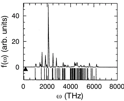
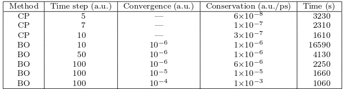
In order to shed light on the title question, the dynamics generated by the Car– Parrinello Lagrangian Eq. (41) is analyzed 467 in more detail invoking a “classical dynamics perspective” of a simple model system (eight silicon atoms forming a periodic diamond lattice, local density approximation to density functional theory, normconserving pseudopotentials for core electrons, plane wave basis for valence orbitals, 0.3 fs time step withµ = 300 a.u., in total 20 000 time steps or 6.3 ps), for full details see Ref. 467); a concise presentation of similar ideas can be found in Ref. 110. For this system the vibrational density of states or power spectrum
of the electronic degrees of freedom, i.e. the Fourier transform of the statistically averaged velocity autocorrelation function of the classical fields
f(ω) =
Z ∞
0
dtcos(ωt)X i
D
˙
ψi;t
ψ˙i; 0
E
(47)
is compared to the highest–frequency phonon modeωmax
n of the nuclear subsystem
in Fig. 2. From this figure it is evident that for the chosen parameters the nuclear and electronic subsystems are dynamically separated: their power spectra do not overlap so that energy transfer from the hot to the cold subsystem is expected to be prohibitively slow, see Sect. 3.3 in Ref. 513for a similar argument.
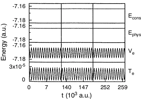
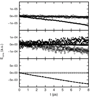
This is indeed the case as can be verified in Fig. 3 where the conserved energy
4 0
Figure 2. Vibrational density of states Eq. (47) (continuous spectrum in upper part) and harmonic approximation thereof Eq. (52) (stick spectrum in lower part) of the electronic degrees of freedom compared to the highest–frequency phonon modeωmax
n (triangle) for a model system; for further
details see text. Adapted from Ref.467
.
of the electronsTe
Econs=
are shown for the same system as a function of time. First of all, there should be a conserved energy quantity according to classical dynamics since the constraints are holonomic244. Indeed “the Hamiltonian” or conserved energyE
consis a constant of
motion (with relative variations smaller than 10−6and with no drift), which serves
as an extremely sensitive check of the molecular dynamics algorithm. Contrary to that the electronic energy Ve displays a simple oscillation pattern due to the
simplicity of the phonon modes.
Most importantly, the fictitious kinetic energy of the electrons Te is found to
perform boundoscillations around aconstant, i.e. the electrons “do not heat up” systematically in the presence of the hot nuclei; note thatTe is a measure for
devi-ations from the exact Born–Oppenheimer surface. Closer inspection shows actually two time scales of oscillations: the one visible in Fig. 3 stems from the drag exerted by the moving nuclei on the electrons and is the mirror image of theVefluctuations.
0
0 7 1 4 0 1 4 7 2 5 2 2 5 9 3 x 1 0 - 5
- 7 . 1 8 - 7 . 1 8 - 7 . 1 6 - 7 . 1 8 - 7 . 1 6 - 7 . 1 6
t ( 1 0 3 a . u . )
E
n
e
rg
y
(
a
.u
.)
E c o n s
E p h y s
V e
T e
Figure 3. Various energies Eqs. (48)–(51) for a model system propagated via Car–Parrinello molec-ular dynamics for at short (up to 300 fs), intermediate, and long times (up to 6.3 ps); for further details see text. Adapted from Ref.467
.
for the stability of the Car–Parrinello dynamics, vide infra. But already the visible variations are three orders of magnitude smaller than the physically meaningful os-cillations ofVe. As a result,Ephys defined asEcons−Te or equivalently as the sum
of the nuclear kinetic energy and the electronic total energy (which serves as the potential energy for the nuclei) is essentially constant on the relevant energy and time scales. Thus, it behaves approximately like the strictly conserved total energy in classical molecular dynamics (with only nuclei as dynamical degrees of freedom) or in Born–Oppenheimer molecular dynamics (with fully optimized electronic de-grees of freedom) and is therefore often denoted as the “physical total energy”. This implies that the resulting physically significant dynamics of the nuclei yields an excellent approximation to microcanonical dynamics (and assuming ergodicity to the microcanonical ensemble). Note that a different explanation was advocated in Ref.470(see also Ref.472, in particular Sect. VIII.B and C), which was however
revised in Ref. 110. A discussion similar in spirit to the one outlined here 467 is
provided in Ref. 513, see in particular Sect. 3.2 and 3.3.
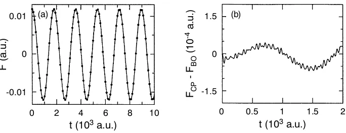
Given the adiabatic separation and the stability of the propagation, the central question remains if the forces acting on the nuclei are actually the “correct” ones in Car–Parrinello molecular dynamics. As a reference serve the forces obtained from full self–consistent minimizations of the electronic energy min{ψi}hΨ0|He|Ψ0i at each time step, i.e. Born–Oppenheimer molecular dynamics with extremely well converged wavefunctions. This is indeed the case as demonstrated in Fig. 4(a): the physically meaningful dynamics of the x–component of the force acting on one silicon atom in the model system obtained from stable Car–Parrinello fictitious dynamics propagation of the electrons and from iterative minimizations of the elec-tronic energy are extremely close.
0
0 . 0 1
- 0 . 0 1
0 2 4 6 8 1 0
( a )
t ( 1 0 3 a . u . )
F
(
a
.u
.)
0 0 . 5 1 1 . 5 2
1 . 5
0
- 1 . 5
t ( 1 0 3 a . u . )
FC
P
F
B
O
(
1
0
-4 a
.u
.) ( b )
Figure 4. (a) Comparison of thex–component of the force acting on one atom of a model system obtained from Car–Parrinello (solid line) and well–converged Born–Oppenheimer (dots) molecular dynamics. (b) Enlarged view of the difference between Car–Parrinello and Born–Oppenheimer forces; for further details see text. Adapted from Ref.467
.
the physical variations of the force resolved in Fig. 4(a). These correspond to the “large–amplitude” oscillations of Te visible in Fig. 3 due to the drag of the nuclei
exerted on the quasi–adiabatically following electrons having a finite dynamical massµ. Note that the inertia of the electrons also dampens artificially the nuclear motion (typically on a few–percent scale, see Sect. V.C.2 in Ref. 75 for an
anal-ysis and a renormalization correction of MI) but decreases as the fictitious mass approaches the adiabatic limitµ→0. Superimposed on the gross variation in (b) are again high–frequencybound oscillatory small–amplitudefluctuations like forTe.
They leadon physically relevant time scales(i.e. those visible in Fig. 4(a)) to “av-eraged forces” that are very close to the exact ground–state Born–Oppenheimer forces. This feature is an important ingredient in the derivation of adiabatic dy-namics467,411.
In conclusion, the Car–Parrinello force can be said to deviate at most instants of time from the exact Born–Oppenheimer force. However, this does not disturb the physical time evolution due to (i) the smallness and boundedness of this difference
and(ii) the intrinsic averaging effect of small–amplitude high–frequency oscillations within a few molecular dynamics time steps, i.e. on the sub–femtosecond time scale which is irrelevant fornuclear dynamics.
2.4.4 How to Control Adiabaticity ?
An important question is under which circumstances the adiabatic separation can be achieved, and how it can be controlled. A simple harmonic analysis of the frequency spectrum of the orbital classical fields close to the minimum defining the ground state yields467
ωij =
2(ǫi−ǫj)
µ
1/2
where ǫj and ǫi are the eigenvalues of occupied and unoccupied orbitals, respec-tively; see Eq. (26) in Ref. 467for the case where both orbitals are occupied ones.
It can be seen from Fig. 2 that the harmonic approximation works faithfully as compared to the exact spectrum; see Ref.471and Sect. IV.A in Ref.472for a more
general analysis of the associated equations of motion. Since this is in particu-lar true for the lowest frequency ωmin
e , the handy analytic estimate for the lowest
possible electronic frequency
ωmin
e ∝
E
gap
µ
1/2
, (53)
shows that this frequency increases like the square root of the electronic energy difference Egap between the lowest unoccupied and the highest occupied orbital.
On the other hand it increases similarly for a decreasing fictitious mass parameter
µ.
In order to guarantee the adiabatic separation, the frequency differenceωmin
e −
ωmax
n should be large, see Sect. 3.3 in Ref. 513 for a similar argument. But both
the highest phonon frequency ωmax
n and the energy gapEgapare quantities that a
dictated by the physics of the system. Whence, the only parameter in our hands to control adiabatic separation is the fictitious mass, which is therefore also called “adiabaticity parameter”. However, decreasing µ not only shifts the electronic spectrum upwards on the frequency scale, but also stretches the entire frequency spectrum according to Eq. (52). This leads to an increase of the maximum frequency according to
ωmax
e ∝
E
cut
µ
1/2
, (54)
where Ecut is the largest kinetic energy in an expansion of the wavefunction in
terms of a plane wave basis set, see Sect. 3.1.3.
At this place a limitation to decreaseµarbitrarily kicks in due to the maximum length of the molecular dynamics time step ∆tmaxthat can be used. The time step
is inversely proportional to the highest frequency in the system, which isωmax
e and
thus the relation
∆tmax∝
µ Ecut
1/2
(55)
governs the largest time step that is possible. As a consequence, Car–Parrinello simulators have to find their way between Scylla and Charybdis and have to make a compromise on the control parameter µ; typical values for large–gap systems are
µ = 500–1500 a.u. together with a time step of about 5–10 a.u. (0.12–0.24 fs). Recently, an algorithm was devised that optimizesµduring a particular simulation given a fixed accuracy criterion 87. Note that a poor man’s way to keep the time
step large and still increase µin order to satisfy adiabaticity is to choose heavier nuclear masses. That depresses the largest phonon or vibrational frequency ωmax
n
Up to this point the entire discussion of the stability and adiabaticity issues was based on model systems, approximate and mostly qualitative in nature. But recently it was actually proven86that the deviation or the absolute error ∆
µ of the Car–Parrinello trajectory relative to the trajectory obtained on the exact Born– Oppenheimer potential energy surface is controlled byµ:
Theorem 1 iv.): There are constants C >0and µ⋆ >0such that
∆µ=
Rµ(t)−R0(t)+|ψµ;ti −ψ0;t≤Cµ1/2 , 0≤t≤T (56)
and the fictitious kinetic energy satisfies
Te=
1 2µ
D
˙
ψµ;t
ψ˙µ;t
E
≤Cµ , 0≤t≤T (57)
for all values of the parameter µ satisfying 0< µ≤ µ⋆,where up to timeT > 0 there exists a unique nuclear trajectory on the exact Born–Oppenheimer surface with ωmin
e > 0 for 0≤ t≤ T, i.e. there is “always” a finite electronic excitation
gap. Here, the superscript µ or 0 indicates that the trajectory was obtained via Car–Parrinello molecular dynamics using a finite mass µ or via dynamics on the exact Born–Oppenheimer surface, respectively. Note that not only the nuclear trajectory is shown to be close to the correct one, but also the wavefunction is proven to stay close to the fully converged one up to time T. Furthermore, it was also investigated what happens if the initial wavefunction at t= 0 is not the minimum of the electronic energyhHeibut trapped in an excited state. In this case
it is found that the propagated wavefunction will keep on oscillating att >0 also forµ→0 and not even time averages converge to any of the eigenstates. Note that this does not preclude Car–Parrinello molecular dynamics in excited states, which is possible given a properly “minimizable” expression for the electronic energy, see e.g. Refs. 281,214. However, this finding might have crucial implications for electronic
level–crossing situations.
What happens if the electronic gap is very small or even vanishes Egap → 0
as is the case for metallic systems? In this limit, all the above–given arguments break down due to the occurrence of zero–frequency electronic modes in the power spectrum according to Eq. (53), which necessarily overlap with the phonon spec-trum. Following an idea of Sprik 583 applied in a classical context it was shown
that the coupling of separate Nos´e–Hoover thermostats12,270,217to the nuclear and
electronic subsystem can maintain adiabaticity by counterbalancing the energy flow from ions to electrons so that the electrons stay “cool” 74; see Ref.204 for a
simi-lar idea to restore adiabaticity. Although this method is demonstrated to work in practice464, thisad hoccure is not entirely satisfactory from both a theoretical and
practical point of view so that the well–controlled Born–Oppenheimer approach is recommended for strongly metallic systems. An additional advantage for metal-lic systems is that the latter is also better suited to sample many k–points (see Sect. 3.1.3), allows easily for fractional occupation numbers 458,168, and can handle
2.4.5 The Quantum Chemistry Viewpoint
In order to understand Car–Parrinello molecular dynamics also from the “quantum chemistry perspective”, it is useful to formulate it for the special case of the Hartree– Fock approximation using
The resulting equations of motion
MIR¨I(t) =−∇IΨ0
are very close to those obtained for Born–Oppenheimer molecular dynamics Eqs. (39)–(40) except for (i) no need to minimize the electronic total energy ex-pression and (ii) featuring the additional fictitious kinetic energy term associated to the orbital degrees of freedom. It is suggestive to argue that both sets of equa-tions become identical if the term |µiψ¨i(t)|is small at any timet compared to the physically relevant forces on the right–hand–side of both Eq. (59) and Eq. (60). This term being zero (or small) means that one is at (or close to) the minimum of the electronic energy hΨ0|HHFe |Ψ0isince time derivatives of the orbitals{ψi}can be considered as variations of Ψ0 and thus of the expectation value hHHFe i itself.
In other words, no forces act on the wavefunction ifµiψ¨i ≡0. In conclusion, the Car–Parrinello equations are expected to produce the correct dynamics and thus physical trajectories in the microcanonical ensemble in this idealized limit. But if |µiψ¨i(t)| is small for all i, this also implies that the associated kinetic energy
Te = Piµihψ˙i|ψ˙ii/2 is small, which connects these more qualitative arguments with the previous discussion 467.
At this stage, it is also interesting to compare the structure of the Lagrangian Eq. (58) and the Euler–Lagrange equation Eq. (43) for Car–Parrinello dynamics to the analogues equations (36) and (37), respectively, used to derive “Hartree–Fock statics”. The former reduce to the latter if the dynamical aspect and the associated time evolution is neglected, that is in the limit that the nuclear and electronic momenta are absent or constant. Thus, the Car–Parrinello ansatz, namely Eq. (41) together with Eqs. (42)–(43), can also be viewed as a prescription to derive a new class of “dynamicalab initiomethods” in very general terms.
2.4.6 The Simulated Annealing and Optimization Viewpoints
In the discussion given above, Car–Parrinello molecular dynamics was motivated by “combining” the positive features of both Ehrenfest and Born–Oppenheimer molecular dynamics as much as possible. Looked at from another side, the Car– Parrinello method can also be considered as an ingenious way to perform global
optimizations (minimizations) of nonlinear functions, here hΨ0|He|Ψ0i, in a high–
parameters are those used to represent the total wavefunction Ψ0in terms of simpler
functions, for instance expansion coefficients of the orbitals in terms of Gaussians or plane waves, see e.g. Refs. 583,375,693,608 for applications of the same idea in
other fields.
Keeping the nuclei frozen for a moment, one could start this optimization pro-cedure from a “random wavefunction” which certainly does not minimize the elec-tronic energy. Thus, its fictitious kinetic energy is high, the elecelec-tronic degrees of freedom are “hot”. This energy, however, can be extracted from the system by systematically cooling it to lower and lower temperatures. This can be achieved in an elegant way by adding a non–conservative damping term to the electronic Car–Parrinello equation of motion Eq. (45)
µiψ¨i(t) =− δ
δψ⋆ i h
Ψ0|He|Ψ0i+ δ
δψ⋆ i {
constraints} −γeµiψi , (61)
where γe≥0 is a friction constant that governs the rate of energy dissipation 610;
alternatively, dissipation can be enforced in a discrete fashion by reducing the veloc-ities by multiplying them with a constant factor <1. Note that this deterministic and dynamical method is very similar in spirit to simulated annealing332 invented
in the framework of the stochastic Monte Carlo approach in the canonical ensemble. If the energy dissipation is done slowly, the wavefunction will find its way down to the minimum of the energy. At the end, an intricate global optimization has been performed!
If the nuclei are allowed to move according to Eq. (44) in the presence of an-other damping term a combined or simultaneous optimization of both electrons and nuclei can be achieved, which amounts to a “global geometry optimization”. This perspective is stressed in more detail in the review Ref. 223 and an
imple-mentation of such ideas within theCADPACquantum chemistry code is described in Ref.692. This operational mode of Car–Parrinello molecular dynamics is related to
other optimization techniques where it is aimed to optimize simultaneously both the structure of the nuclear skeleton and the electronic structure. This is achieved by considering the nuclear coordinates and the expansion coefficients of the orbitals as variation parameters on the same footing 49,290,608. But Car–Parrinello molecular
dynamics is more than that because even if the nuclei continuously move according to Newtonian dynamics at finite temperature an initially optimized wavefunction will stay optimal along the nuclear trajectory.
2.4.7 The Extended Lagrangian Viewpoint
There is still another way to look at the Car–Parrinello method, namely in the light of so–called “extended Lagrangians” or “extended system dynamics” 14, see
e.g. Refs.136,12,270,585,217for introductions. The basic idea is to couple additional
The corresponding equations of motion follow from the Euler–Lagrange equa-tions and yield a microcanonical ensemble in the extended phase space where the Hamiltonian of the extended system is strictly conserved. In other words, the Hamiltonian of the physical (sub–) system is no more (strictly) conserved, and the produced ensemble is no more the microcanonical one. Any extended system dy-namics is constructed such that time–averages taken in that part of phase space that is associated to the physical degrees of freedom (obtained from a partial trace over the fictitious degrees of freedom) are physically meaningful. Of course, dynamics and thermodynamics of the system are affected by adding fictitious degrees of free-dom, the classic examples being temperature and pressure control by thermostats and barostats, see Sect. 4.2.
In the case of Car–Parrinello molecular dynamics, the basic Lagrangian for Newtonian dynamics of the nuclei is actually extended by classical fields{ψi(r)}, i.e. functions instead of coordinates, which represent the quantum wavefunction. Thus, vector products or absolute values have to be generalized to scalar products and norms of the fields. In addition, the “positions” of these fields {ψi}actually have a physical meaning, contrary to their momenta{ψ˙i}.
2.5 What about Hellmann–Feynman Forces ?
An important ingredient in all dynamics methods is the efficient calculation of the forces acting on the nuclei, see Eqs. (30), (32), and (44). The straightforward numerical evaluation of the derivative
FI =−∇IhΨ0|He|Ψ0i (62)
in terms of a finite–difference approximation of the total electronic energy is both too costly and too inaccurate for dynamical simulations. What happens if the gra-dients are evaluated analytically? In addition to the derivative of the Hamiltonian itself
∇IhΨ0|He|Ψ0i=hΨ0|∇IHe|Ψ0i
+h∇IΨ0|He|Ψ0i+hΨ0|He|∇IΨ0i (63)
there are in general also contributions from variations of the wavefunction∼ ∇IΨ0.
In general means here that these contributions vanish exactly
FHFTI =− hΨ0|∇IHe|Ψ0i (64)
if the wavefunction is an exact eigenfunction (or stationary state wavefunction) of the particular Hamiltonian under consideration. This is the content of the often– cited Hellmann–Feynman Theorem 295,186,368, which is also valid for many
varia-tional wavefunctions (e.g. the Hartree–Fock wavefunction) provided thatcomplete basis sets are used. If this is not the case, which has to be assumed for numerical calculations, the additional terms have to be evaluated explicitly.
In order to proceed a Slater determinant Ψ0= det{ψi}of one–particle orbitals
ψi, which themselves are expanded
ψi=
X
ν
in terms of a linear combination of basis functions{fν}, is used in conjunction with an effective one–particle Hamiltonian (such as e.g. in Hartree–Fock or Kohn–Sham theories). The basis functions might depend explicitly on the nuclear positions (in the case of basis functions with origin such as atom–centered orbitals), whereas the expansion coefficients always carry an implicit dependence. This means that from the outset two sorts of forces are expected
∇Iψi=
X
ν
(∇Iciν) fν(r;{RI}) +
X
ν
ciν (∇Ifν(r;{RI})) (66) in addition to the Hellmann–Feynman force Eq. (64).
Using such a linear expansion Eq. (65), the force contributions stemming from the nuclear gradients of the wavefunction in Eq. (63) can be disentangled into two terms. The first one is called “incomplete–basis–set correction” (IBS) in solid state theory49,591,180and corresponds to the “wavefunction force”494or “Pulay force” in
quantum chemistry 494,496. It contains the nuclear gradients of the basis functions
FIBSI =−X
iνµ
∇IfνHNSCe −ǫifµ+fνHNSCe −ǫi∇fµ (67)
and the (in practice non–self–consistent) effective one–particle Hamiltonian49,591.
The second term leads to the so–called “non–self–consistency correction” (NSC) of the force49,591
FNSCI =−
Z
dr(∇In) VSCF−VNSC (68) and is governed by the difference between the self–consistent (“exact”) potential or field VSCF and its non–self–consistent (or approximate) counterpart VNSC
associ-ated toHNSC
e ;n(r) is the charge density. In summary, the total force needed inab initiomolecular dynamics simulations
FI =FHFTI +FIBSI +FNSCI (69) comprises in general three qualitatively different terms; see the tutorial article Ref.180for a further discussion of core vs. valence states and the effect of
pseudopo-tentials. Assuming that self–consistency is exactly satisfied (which is never going to be the case in numerical calculations), the forceFNSC
I vanishes andHSCFe has to
be used to evaluate FIBS
I . The Pulay contribution vanishes in the limit of using a complete basis set (which is also not possible to achieve in actual calculations).
The most obvious simplification arises if the wavefunction is expanded in terms of originless basis functions such as plane waves, see Eq. (100). In this case the Pu-lay force vanishes exactly, which applies of course to allab initiomolecular dynamics schemes (i.e. Ehrenfest, Born–Oppenheimer, and Car–Parrinello) using that par-ticular basis set. This statement is true for calculations where the number of plane waves is fixed. If the number of plane waves changes, such as in (constant pressure) calculations with varying cell volume / shape where the energy cutoff is strictly fixed instead, Pulay stress contributions crop up 219,245,660,211,202, see Sect. 4.2. If
basis sets with origin are used instead of plane waves Pulay forces arise always and have to be included explicitely in force calculations, see e.g. Refs. 75,370,371for such
there is no basis set superposition error (BSSE) 88 in plane wave–based electronic
structure calculations.
A non–obvious and more delicate term in the context of ab initio molecular dynamics is the one stemming from non–self–consistency Eq. (68). This term van-ishes only if the wavefunction Ψ0 is an eigenfunction of the Hamiltonianwithin the subspace spanned by the finite basis set used. This demands less than the Hellmann– Feynman theorem where Ψ0 has to be an exact eigenfunction of the Hamiltonian
and a complete basis set has to be used in turn. In terms of electronic structure calculations complete self–consistency (within a given incomplete basis set) has to be reached in order thatFNSC
I vanishes. Thus, in numerical calculations the NSC term can be made arbitrarily small by optimizing the effective Hamiltonian and by determining its eigenfunctions to very high accuracy, but it can never be suppressed completely.
The crucial point is, however, that in Car–Parrinello as well as in Ehrenfest molecular dynamics it is not the minimized expectation value of the electronic Hamiltonian, i.e. minΨ0{hΨ0|He|Ψ0i}, that yields the consistent forces. What is
merely needed is to evaluate the expression hΨ0|He|Ψ0iwith the Hamiltonian and
the associated wavefunction available at a certain time step, compare Eq. (32) to Eq. (44) or (30). In other words, it is not required (concerning the present discussion of the contributions to the force!) that the expectation value of the electronic Hamiltonian is actually completely minimized for the nuclear configuration at that time step. Whence, full self–consistency is not required for this purpose in the case of Car–Parrinello (and Ehrenfest) molecular dynamics. As a consequence, the non– self–consistency correction to the forceFNSC
I Eq. (68) is irrelevant in Car–Parrinello (and Ehrenfest) simulations.
In Born–Oppenheimer molecular dynamics, on the other hand, the expectation value of the Hamiltonian has to be minimized for each nuclear configuration before taking the gradient to obtain the consistent force! In this scheme there is (inde-pendently from the issue of Pulay forces)always the non–vanishing contribution of the non–self–consistency force, which is unknown by its very definition (if it were know, the problem was solved, see Eq. (68)). It is noted in passing that there are estimation schemes available that correctapproximatelyfor this systematic error in Born–Oppenheimer dynamics and lead to significant time–savings, see e.g. Ref.344.
Heuristically one could also argue that within Car–Parrinello dynamics the non– vanishing non–self–consistency force is kept under control or counterbalanced by the non–vanishing “mass times acceleration term” µiψ¨i(t)≈0, which is small but not identical to zero and oscillatory. This is sufficient to keep the propagation sta-ble, whereasµiψ¨i(t)≡0, i.e. an extremely tight minimization minΨ0{hΨ0|He|Ψ0i},
is required by its very definition in order to make the Born–Oppenheimer approach stable, compare again Eq. (60) to Eq. (40). Thus, also from this perspective it becomes clear that the fictitious kinetic energy of the electrons and thus their ficti-tious temperature is a measure for the departure from the exact Born–Oppenheimer surface during Car–Parrinello dynamics.
Finally, the present discussion shows that nowhere in these force derivations was
structure calculations, see e.g. Refs. 494,49,496 and references therein. Rather it turns out that in the case of Car–Parrinello calculations using a plane wave basis the resulting relation for the force, namely Eq. (64), looks like the one obtained by simply invoking the Hellmann–Feynman theorem at the outset.
It is interesting to recall that the Hellmann–Feynman theorem as applied to a non–eigenfunction of a Hamiltonian yields only a first–order perturbative estimate of the exact force 295,368. The same argument applies to ab initiomolecular
dy-namics calculations where possible force corrections according to Eqs. (67) and (68) are neglected without justification. Furthermore, such simulations can of course not strictly conserve the total HamiltonianEconsEq. (48). Finally, it should be stressed
that possible contributions to the force in the nuclear equation of motion Eq. (44) due to position–dependent wavefunctionconstraintshave to be evaluated following the same procedure. This leads to similar “correction terms” to the force, see e.g. Ref. 351for such a case.
2.6 Which Method to Choose ?
Presumably the most important question for practical applications is whichab initio
molecular dynamics method is the most efficient in terms of computer time given a specific problem. An a prioriadvantage of both the Ehrenfest and Car–Parrinello schemes over Born–Oppenheimer molecular dynamics is that no diagonalization of the Hamiltonian (or the equivalent minimization of an energy functional) is necessary, except at the very first step in order to obtain the initial wavefunc-tion. The difference is, however, that the Ehrenfest time–evolution according to the time–dependent Schr¨odinger equation Eq. (26) conforms to a unitary propaga-tion341,366,342
Ψ(t0+ ∆t) = exp [−iHe(t0)∆t/ ] Ψ(t0) (70)
Ψ(t0+m∆t) = exp [−iHe(t0+ (m−1)∆t) ∆t/ ]
× · · ·
×exp [−iHe(t0+ 2∆t) ∆t/ ]
×exp [−iHe(t0+ ∆t) ∆t/ ]
×exp [−iHe(t0) ∆t/ ] Ψ(t0) (71)
Ψ(t0+tmax)
∆t→0
= Texp
"
−i
Z t0+tmax
t0
dtHe(t) #
Ψ(t0) (72)
for infinitesimally short times given by the time step ∆t=tmax/m; here
T is the time–ordering operator and He(t) is the Hamiltonian (which is implicitly time–
dependent via the positions {RI(t)}) evaluated at time tusing e.g. split operator techniques 183. Thus, the wavefunction Ψ will conserve its norm and in particular
orbitals used to expand it will stay orthonormal, see e.g. Ref.617. In Car–Parrinello