Introduction to
Simulation Modeling
Simulation modeling is a common paradigm for analyzing complex systems. In a nutshell, this paradigm creates a simplified representation of a system under study. The paradigm then proceeds to experiment with the system, guided by a prescribed set of goals, such as improved system design, cost–benefit analysis, sensitivity to design parameters, and so on. Experimentation consists of generating system histories and observing system behavior over time, as well as its statistics. Thus, the representation created (see Section 1.1) describes system structure, while the histories generated describe system behavior (see Section 1.5).
This book is concerned with simulation modeling of industrial systems. Included are manufacturing systems (e.g., production lines, inventory systems, job shops, etc.), supply chains, computer and communications systems (e.g., client-server systems, communi-cations networks, etc.), and transportation systems (e.g., seaports, airports, etc.). The book addresses both theoretical topics and practical ones related to simulation modeling. Throughout the book, the Arena/SIMAN (see Keltonet al. 2000) simulation tool will be surveyed and used in hands-on examples of simulation modeling.
This chapter overviews the elements of simulation modeling and introduces basic concepts germane to such modeling.
1.1
SYSTEMS AND MODELS
Modeling is the enterprise of devising a simplified representation of a complex system with the goal of providing predictions of the system's performance measures (metrics) of interest. Such a simplified representation is called a model. A model is designed to capture certain behavioral aspects of the modeled system—those that are of interest to the analyst/modeler—in order to gain knowledge and insight into the system's behavior (Morris 1967).
Modeling calls for abstraction and simplification. In fact, if every facet of the system under study were to be reproduced in minute detail, then the model cost may approach that of the modeled system, thereby militating against creating a model in the first place.
Simulation Modeling and Analysis with Arena
The modeler would simply use the “real” system or build an experimental one if it does not yet exist—an expensive and tedious proposition. Models are typically built precisely to avoid this unpalatable option. More specifically, while modeling is ultim-ately motivated by economic considerations, several motivational strands may be discerned:
Evaluating system performance under ordinary and unusual scenarios. A model may
be a necessity if the routine operation of the real-life system under study cannot be disrupted without severe consequences (e.g., attempting an upgrade of a production line in the midst of filling customer orders with tight deadlines). In other cases, the extreme scenario modeled is to be avoided at all costs (e.g., think of modeling a crash-avoiding maneuver of manned aircraft, or core meltdown in a nuclear reactor).
Predicting the performance of experimental system designs. When the underlying
system does not yet exist, model construction (and manipulation) is far cheaper (and safer) than building the real-life system or even its prototype. Horror stories appear periodically in the media on projects that were rushed to the implementation phase, without proper verification that their design is adequate, only to discover that the system was flawed to one degree or another (recall the case of the brand new airport with faulty luggage transport).
Ranking multiple designs and analyzing their tradeoffs. This case is related to the
previous one, except that the economic motivation is even greater. It often arises when the requisition of an expensive system (with detailed specifications) is awarded to the bidder with the best cost–benefit metrics.
Models can assume a variety of forms:
Aphysical modelis a simplified or scaled-down physical object (e.g., scale model of an
airplane).
Amathematicaloranalytical modelis a set of equations or relations among
mathemat-ical variables (e.g., a set of equations describing the workflow on a factory floor).
Acomputer modelis just a program description of the system. A computer model with
random elements and an underlying timeline is called aMonte Carlo simulation model
(e.g., the operation of a manufacturing process over a period of time).
Monte Carlo simulation, orsimulationfor short, is the subject matter of this book. We shall be primarily concerned with simulation models of production, transportation, and computer information systems. Examples include production lines, inventory systems, tollbooths, port operations, and database systems.
1.2
ANALYTICAL VERSUS SIMULATION MODELING
A simulation model is implemented in a computer program. It is generally a relatively inexpensive modeling approach, commonly used as an alternative to analytical model-ing. The tradeoff between analytical and simulation modeling lies in the nature of their
“solutions,”that is, the computation of their performance measures as follows:
2. A simulation model calls for running (executing) a simulation program to produce sample histories. A set of statisticscomputed from these histories is then used to form performance measures of interest.
To compare and contrast both approaches, suppose that a production line is concep-tually modeled as a queuing system. The analytical approach would create an analytical queuing system (represented by a set of equations) and proceed to solve them. The simulation approach would create a computer representation of the queuing system and run it to produce a sufficient number of sample histories. Performance measures, such as average work in the system, distribution of waiting times, and so on, would be constructed from the corresponding“solutions”as mathematical or simulation statistics, respectively.
The choice of an analytical approach versus simulation is governed by general tradeoffs. For instance, an analytical model ispreferableto a simulation model when it has a solution, since its computation is normally much faster than that of its simula-tion-model counterpart. Unfortunately, complex systems rarely lend themselves to modeling via sufficiently detailed analytical models. Occasionally, though rarely, the numerical computation of an analytical solution is actually slower than a corresponding simulation. In the majority of cases, an analytical model with a tractable solution is unknown, and the modeler resorts to simulation.
When the underlying system is complex, a simulation model is normallypreferable, for several reasons. First, in the unlikely event that an analytical model can be found, the modeler's time spent in deriving a solution may be excessive. Second, the modeler may judge that an attempt at an analytical solution is a poor bet, due to the apparent mathematical difficulties. Finally, the modeler may not even be able to formulate an analytical model with sufficient power to capture the system's behavioral aspects of interest. In contrast, simulation modeling can capture virtually any system, subject to any set of assumptions. It also enjoys the advantage of dispensing with the labor attendant to finding analytical solutions, since the modeler merely needs to construct and run a simulation program. Occasionally, however, the effort involved in construct-ing an elaborate simulation model is prohibitive in terms of human effort, or runnconstruct-ing the resultant program is prohibitive in terms of computer resources (CPU time and memory). In such cases, the modeler must settle for a simpler simulation model, or even an inferior analytical model.
Another way to contrast analytical and simulation models is via the classification of models intodescriptiveorprescriptive models. Descriptive models produce estimates for a set of performance measures corresponding to a specific set of input data. Simulation models are clearly descriptive and in this sense serve as performance analysis models. Prescriptive models are naturally geared toward design or optimization (seeking the optimal argument values of a prescribed objective function, subject to a set of constraints). Analytical models are prescriptive, whereas simulation is not. More specifically, analytical methods can serve as effective optimization tools, whereas simulation-based optimization usually calls for an exhaustive search for the optimum.
In particular, the complexity of industrial and service systems often forces the issue of selecting simulation as the modeling methodology of choice.
1.3
SIMULATION MODELING AND ANALYSIS
The advent of computers has greatly extended the applicability of practical simula-tion modeling. Since World War II, simulasimula-tion has become an indispensable tool in many system-related activities. Simulation modeling has been applied to estimate performance metrics, to answer“what if”questions, and more recently, to train workers in the use of new systems. Examples follow.
Estimating a set of productivity measures in production systems, inventory systems,
manufacturing processes, materials handling, and logistics operations
Designing and planning the capacity of computer systems and communication networks
so as to minimize response times
Conducting war games to train military personnel or to evaluate the efficacy of
proposed military operations
Evaluating and improving maritime port operations, such as container ports or
bulk-material marine terminals (coal, oil, or minerals), aimed at finding ways of reducing vessel port times
Improving health care operations, financial and banking operations, and transportation
systems and airports, among many others
In addition, simulation is now used by a variety of technology workers, ranging from design engineers to plant operators and project managers. In particular, manufac-turing-related activities as well as business process reengineering activities employ simulation to select design parameters, plan factory floor layout and equipment pur-chases, and even evaluate financial costs and return on investment (e.g., retooling, new installations, new products, and capital investment projects).
1.4
SIMULATION WORLDVIEWS
Aworldviewis a philosophy or paradigm. Every computer tool has two associated worldviews: a developer worldview and a user worldview. These two worldviews should be carefully distinguished. The first worldview pertains to the philosophy adopted by the creators of the simulation software tool (in our case, software designers and engineers). The second worldview pertains to the way the system is employed as a tool by end-users (in our case, analysts who create simulation models as code written in somesimulation language). A system worldview may or may not coincide with an end-user worldview, but the latter includes the former.
simulation event occurs, at which point the model undergoes a state transition. The model evolution is governed by aclockand a chronologically orderedevent list. Each event is implemented as a procedure (computer code) whose execution can change state variables and possibly schedule other events. A simulation run is started by placing an initial event in the event list, proceeds as an infinite loop that executes the current most imminent event (the one at the head of the event list), and ends when an event stops or the event list becomes empty. This beguilingly simple paradigm is extremely general and astonishingly versatile.
Early simulation languages employed a user worldview that coincided with the discrete-event paradigm. A more convenient, but more specialized, paradigm is the transaction-driven paradigm (commonly referred to as process orientation). In this popular paradigm, there are two kinds of entities:transactions and resources. A resource is a service-providing entity, typically stationary in space (e.g., a machine on the factory floor). A transaction is a mobile entity that moves among“geographical”
locations (nodes). A transaction may experience delays while waiting for a resource due to contention (e.g., a product that moves among machines in the course of assem-bly). Transactions typically go through a life cycle: they get created, spend time at various locations, contend for resources, and eventually depart from the system. The computer code describing a transaction's life cycle is called aprocess.
Queuing elements figure prominently in this paradigm, since facilities typically contain resources and queues. Accordingly, performance measures of interest include statistics of delays in queues, the number of transactions in queues, utilization, uptimes and downtimes of resources subject to failure, and lost demand, among many others.
1.5
MODEL BUILDING
Modeling, including simulation modeling, is a complicated activity that combines art and science. Nevertheless, from a high-level standpoint, one can distinguish the following major steps:
1. Problem analysis and information collection. The first step in building a simula-tion model is to analyze the problem itself. Note that system modeling is rarely undertaken for its own sake. Rather, modeling is prompted by some system-oriented problem whose solution is the mission of the underlying project. In order to facilitate a solution, the analyst first gathers structural information that bears on the problem, and represents it conveniently. This activity includes the identifi-cation of input parameters, performance measures of interest, relationships among parameters and variables, rules governing the operation of system components, and so on. The information is then represented as logic flow diagrams, hierarchy trees, narrative, or any other convenient means of representation. Once sufficient information on the underlying system is gathered, the problem can be analyzed and a solution mapped out.
model validation. That is, data collected on system output statistics are compared to their model counterparts (predictions).
3. Model construction. Once the problem is fully studied and the requisite data collected, the analyst can proceed to construct a model and implement it as a computer program. The computer language employed may be a general-purpose language (e.g., C++, Visual Basic, FORTRAN) or a special-purpose simulation language or environment (e.g., Arena, Promodel, GPSS). See Section 2.4 for details.
4. Model verification. The purpose of model verification is to make sure that the model is correctly constructed. Differently stated, verification makes sure that the model conforms to its specification and does what it is supposed to do. Model verification is conducted largely by inspection, and consists of comparing model code to model specification. Any discrepancies found are reconciled by modifying either the code or the specification.
5. Model validation. Every model should be initially viewed as a mere proposal, subject to validation. Model validation examines the fit of the model to empirical data (measurements of the real-life system to be modeled). A good model fit means here that a set of important performance measures, predicted by the model, match or agree reasonably with their observed counterparts in the real-life system. Of course, this kind of validation is only possible if the real-life system or emulation thereof exists, and if the requisite measurements can actually be acquired. Any significant discrepancies would suggest that the proposed model is inadequate for project purposes, and that modifications are called for. In practice, it is common to go through multiple cycles of model construction, verification, validation, and modification.
6. Designing and conducting simulation experiments. Once the analyst judges a model to be valid, he or she may proceed to design a set of simulation experiments (runs) to estimate model performance and aid in solving the project's problem (often the problem is making system design decisions). The analyst selects a number of scenarios and runs the simulation to glean insights into its workings. To attain sufficient statistical reliability of scenario-related performance measures, each scenario is replicated (run multiple times, subject to different sequences of random numbers), and the results averaged to reduce statistical variability. 7. Output analysis. The estimated performance measures are subjected to a thorough
logical and statistical analysis. A typical problem is one of identifying the best design among a number of competing alternatives. A statistical analysis would run statistical inference tests to determine whether one of the alternative designs enjoys superior performance measures, and so should be selected as the apparent best design.
8. Final recommendations. Finally, the analyst uses the output analysis to formulate the final recommendations for the underlying systems problem. This is usually part of a written report.
1.6
SIMULATION COSTS AND RISKS
Modeling cost. Like any other modeling paradigm, good simulation modeling is a
prerequisite to efficacious solutions. However, modeling is frequently more art than science, and the acquisition of good modeling skills requires a great deal of practice and experience. Consequently, simulation modeling can be a lengthy and costly process. This cost element is, however, a facet of any type of modeling. As in any modeling enterprise, the analyst runs the risk of postulating an inaccurate or patently wrong model, whose invalidity failed to manifest itself at the validation stage. Another pitfall is a model that incorporates excessive detail. The right level of detail depends on the underlying problem. The art of modeling involves the construction of the least-detailed model that can do the job (producing adequate answers to questions of interest).
Coding cost. Simulation modeling requires writing software. This activity can be
error-prone and costly in terms of time and human labor (complex software projects are notorious for frequently failing to complete on time and within budget). In addition, the ever-present danger of incorrect coding calls for meticulous and costly verification.
Simulation runs. Simulation modeling makes extensive use of statistics. The analyst
should be careful to design the simulation experiments, so as to achieve adequate statistical reliability. This means that both the number of simulation runs (replications) and their length should be of adequate magnitude. Failing to do so is to risk the statistical reliability of the estimated performance measures. On the other hand, some simulation models may require enormous computing resources (memory space and CPU time). The modeler should be careful not to come up with a simulation model that requires prohibi-tive computing resources (clever modeling and clever code writing can help here).
Output analysis. Simulation output must be analyzed and properly interpreted.
Incor-rect predictions, based on faulty statistical analysis, and improper understanding of system behavior are ever-present risks.
1.7
EXAMPLE: A PRODUCTION CONTROL PROBLEM
This section presents a simple production control problem as an example of the kind of systems amenable to simulation modeling. This example illustrates system definition and associated performance issues. A variant of this system will be discussed in Section 11.3, and its Arena model will be presented there.
Consider a packaging/warehousing process with the following steps:
1. The product is filled and sealed.
2. Sealed units are placed into boxes and stickers are placed on the boxes. 3. Boxes are transported to the warehouse to fulfill customer demand.
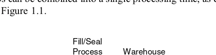
These steps can be combined into a single processing time, as depicted in the system schematic of Figure 1.1.
Warehouse Fill/Seal
Process
Raw Material
Demand
Lost Customers
The system depicted in Figure 1.1 is subject to the following assumptions:
1. There is always sufficient raw material for the process never tostarve.
2. Processing is carried out in batches, five units to a batch. Finished units are placed in the warehouse. Data collected indicate that unit-processing times are uniformly distributed between 10 and 20 minutes.
3. The process experiencesrandom failures, which may occur at any point in time. Times between failures are exponentially distributed with a mean of 200 minutes. Data collection also showed that repair times are normally distributed, with a mean of 90 minutes and a standard deviation of 45 minutes.
4. The warehouse has a capacity(target level) ofR¼500 units. Processing stops
when the inventory in the warehouse reaches the target level. From this point on, the production process becomesblockedand remains inactive until the inventory level drops to the reorder point, which is assumed to be r¼150 units. The
process restarts with a new batch as soon as the reorder level is down-crossed. This is a convenient policy when a resource needs to be distributed among various types of products. For instance, when our process becomes blocked, it may actually be assigned to another task or product that is not part of our model. 5. Data collection shows that interarrival times between successive customers are
uniformly distributed between 3 and 7 hours, and that individual demand sizes are distributed uniformly between 50 and 100 units. On customer arrival, the inventory is immediately checked. If there is sufficient stock on hand, that demand is promptly satisfied; otherwise, customer demand is either partially satisfied and the rest is lost (that is, the unsatisfied portion represents lost business), or the entire demand is lost, depending on the availability of finished units and the loss policy employed.
This problem is also known as aproduction/inventory problem. We mention, how-ever, that the present example is a gross simplification. More realistic production/ inventory problems have additional wrinkles, including multiple types of products, production setups or startups, and so on. Some design and performance issues and associated performance measures of interest follow:
1. Can we improve the customer service level (percentage of customers whose demand is completely satisfied)?
2. Is the machinery underutilized or overutilized (machine utilization)? 3. Is the maintenance level adequate (downtime probabilities)?
4. What is the tradeoff between inventory level and customer service level?
The previous list is far from being exhaustive, and the actual requisite list will, of course, depend on the problem to be solved.
1.8
PROJECT REPORT
A project report should be clearly and plainly written, so that nontechnical people as well as professionals can understand it. This is particularly true for project conclusions and recommendations, as these are likely to be read by management as part of the decision-making process. Although one can hardly overemphasize the importance of project reporting, the topic of proper reporting is rarely addressed explicitly in the published literature. In practice, analysts learn project-writing skills on the job, typically by example.
A generic simulation project report addresses the model building stages described in Section 1.5, and consists of (at least) the following sections:
Cover page. Includes a project title, author names, date, and contact information in this
order. Be sure to compose a descriptive but pithy project title.
Executive summary. Provides a summary of the problem studied, model findings, and
conclusions.
Table of contents. Lists section headings, figures, and tables with the corresponding
page numbers.
Introduction. Sets up the scene with background information on the system under study
(if any), the objectives of the project, and the problems to be solved. If appropriate, include a brief review of the relevant company, its location, and products and services.
System description. Describes in detail the system to be studied, using prose, charts,
and tables (see Section 1.7). Include all relevant details but no more (the rest of the book and especially Chapters 11–13 contain numerous examples).
Input analysis. Describes empirical data collection and statistical data fitting (see
Section 1.5 and Chapter 7). For example, the Arena Input Analyzer (Section 7.4) provides facilities for fitting distributions to empirical data and statistical tests. More advanced model fitting of stochastic processes to empirical data is described in Chapter 10.
Simulation model description. Describes the modeling approach of the simulation
model, and outlines its structure in terms of its main components, objects, and the operational logic. Be sure to decompose the description of a complex model into manageable-size submodel descriptions. Critical parts of the model should be described in some detail.
Verification and validation. Provides supportive evidence for model goodness via
model verification and validation (see Section 1.5) to justify its use in predicting the performance measures of the system under study (see Chapter 8). To this end, be sure to address at least the following two issues: (1) Does the model appear to run correctly and to provide the relevant statistics (verification)? (2) If the modeled system exists, how close are its statistics (e.g., mean waiting times, utilizations, throughputs, etc.) to the corresponding model estimates (validation)?
Output analysis. Describes simulation model outputs, including run scenarios, number
of replications, and the statistical analysis of simulation-produced observations (see Chapter 9). For example, the Arena Output Analyzer (Section 9.6) provides facilities for data graphing, statistical estimation, and statistical comparisons, while the Arena Process Analyzer (Section 9.7) facilitates parametric analysis of simulation models.
Simulation results. Collects and displays summary statistics of multiple replicated
scenarios. Arena's report facilities provide the requisite summary statistics (numerous reports are displayed in the sequel).
Suggested system modifications (if any). A common motivation for modeling an extant
that produce improvements, such as better performance and reduced costs. Be sure to discuss thoroughly the impact of suggested modifications by quantifying improvements and analyzing tradeoffs where relevant.
Conclusions and recommendations. Summarizes study findings and furnishes a set of
recommendations.
Appendices. Contains any relevant material that might provide undesired digression in
the report body.
Needless to say, the modeler/analyst should not hesitate to customize and modify the previous outlined skeleton as necessary.
EXERCISES
1. Consider an online registration system (e.g., course registration at a university or membership registration in a conference).
a. List the main components of the system and its transactions.
b. How would you define the state and events of each component of the registra-tion system?
c. Which performance measures might be of interest to registrants?
d. Which performance measures might be of interest to the system administrator? e. What data would you collect?
2. The First New Brunswick Savings (FNBS) bank has a branch office with a number of tellers serving customers in the lobby, a teller serving the drive-in line, and a number of service managers serving customers with special requests. The lobby, drive-in, and service managers each have a separate single queue. Customers may join either of the queues (the lobby queue, the drive-in queue, or the service managers’ queue). FNBS is interested in performance evaluation of their customer service operations.
a. What are the random components in the system and their parameters? b. What performance measures would you recommend FNBS to consider? c. What data would you collect and why?
3. Consider the production/inventory system of Section 1.7. Suppose the system produces and stores multiple products.
a. List the main components of the system and its transactions as depicted in Figure 1.1.
b. What are the transactions and events of the system, in view of Figure 1.1? c. Which performance measures might be of interest to customers, and which to
owners?