On the Use of the Genetic Algorithm Filter-Based
Feature Selection Technique for Satellite
Precipitation Estimation
Majid Mahrooghy, Nicolas H. Younan,
Senior Member, IEEE
,
Valentine G. Anantharaj, James Aanstoos, and Shantia Yarahmadian
Abstract—A feature selection technique is used to enhance the precipitation estimation from remotely sensed imagery using an artificial neural network (PERSIANN) and cloud classification system (CCS) method (PERSIANN-CCS) enriched by wavelet fea-tures. The feature selection technique includes a feature similarity selection method and a filter-based feature selection using genetic algorithm (FFSGA). It is employed in this study to find an opti-mal set of features where redundant and irrelevant features are removed. The entropy index fitness function is used to evaluate the feature subsets. The results show that using the feature selection technique not only improves the equitable threat score by almost 7% at some threshold values for the winter season, but also it extremely decreases the dimensionality. The bias also decreases in both the winter (January and February) and summer (June, July, and August) seasons.
Index Terms—Clustering, feature extraction, satellite precipita-tion estimaprecipita-tion (SPE), self-organizing map, unsupervised feature selection.
I. INTRODUCTION
A
CCURATELY estimating precipitation at high spatial and temporal resolutions is valuable in many applications such as precipitation forecasting, climate modeling, flood forecast-ing, hydrology, water resources management, and agriculture [1]. For some applications, such as flood forecasting, accurate precipitation estimation is essential. Even though ground-based equipment, such as weather radars andin siturain gauges, pro-vide reliable and accurate precipitation estimates, they cannot cover all regions of the globe. In addition, their coverage is not spatially and temporally uniform in many areas. Furthermore,Manuscript received August 25, 2011; revised December 3, 2011; accepted January 2, 2012. Date of publication March 21, 2012; date of current version May 29, 2012. This work was supported by the National Aeronau-tics and Space Administration under Grant NNS06AA98B and the National Oceanic and Atmospheric Administration under Grant NA07OAR4170517.
M. Mahrooghy and N. H. Younan are with the Department of Electri-cal Engineering, Mississippi State University, Mississippi State, MS 39762 USA, and are also with the Geosystems Research Institute, Mississippi State University, Mississippi State, MS 39762 USA (e-mail: [email protected]; [email protected]).
V. G. Anantharaj is with the National Center for Computational Sci-ences, Oak Ridge National Laboratory, Oak Ridge, TN 37831 USA (e-mail: [email protected]).
J. Aanstoos is with the Geosystems Research Institute, Mississippi State Uni-versity, Mississippi State, MS 39762 USA (e-mail: [email protected]). S. Yarahmadian is with the Department of Mathematics and Statistics, Mississippi State University, Mississippi State, MS 39762 USA (e-mail: [email protected]).
Color versions of one or more of the figures in this paper are available online at http://ieeexplore.ieee.org.
Digital Object Identifier 10.1109/LGRS.2012.2187513
there are not ground-based facilities to estimate rainfall over oceans. In this regard, satellite-based observation systems can be a solution by regularly monitoring the earth’s environment at sufficient spatial and temporal resolutions over large areas. Sev-eral different satellite precipitation estimation (SPE) algorithms are already in routine use [2].
Feature selection is the process of selecting a subset of the original feature space based on an evaluation criterion to improve the quality of the data [3]. It reduces the dimensionality and complexity by removing irrelevant and redundant features. In addition, it increases the speed of the algorithm, as well as may improve the algorithm performance such as predictive ac-curacy. Different feature selection methods have been proposed for supervised and unsupervised learning systems [3]–[5]. Most of the feature selection methods are based on search procedures. However, there are some other techniques such as the feature similarity selection (FSS) method, developed by Mitra et al.
[6], in which no search process is required.
Search-based feature selection techniques are carried out by subset generation, subset evaluation, stopping criterion, and result validation [3]. Based on a search strategy, the subset gen-eration produces the candidate feature subsets for evaluation. Then, each candidate subset is evaluated by a certain evaluation criterion (fitness function) and compared with the previous best subset. If the new candidate has a better evaluation result, it becomes the best subset. This process is repeated until a given stopping criterion is satisfied [3].
The search-based feature selection methods can be catego-rized into three models: filter, wrapper, and hybrid models. Filter methods evaluate the feature subset by using the inherent characteristic of the data. Since learning algorithms are not in-volved in filter models, these models are computationally cheap and fast [3], [7]. On the contrary, wrapper methods directly use learning algorithms to evaluate the feature subsets. They generally surpass filter methods in terms of prediction accuracy, but, in general, they are computationally more expensive and slower [7]. The hybrid model takes advantage of the other two models by utilizing their different evaluation criteria in the different search stages [3].
In a search-based feature selection, the searching process can be complete, sequential, or random. In the case of a complete search (no optimal feature subset is missed), finding a global optimal feature subset is guaranteed based on the evaluation criterion utilized [3]. However, this kind of a search process is exhaustive or time consuming due to its complexity. In a sequential search, not all possible feature subsets are con-sidered. Hence, the best subset may be trapped to the local
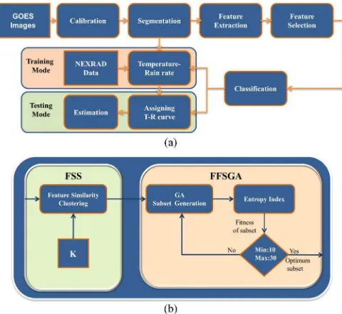
Fig. 1. Block diagram. (a) SPE with feature selection. (b) Feature selection.
optimal subset [3]. These include greedy search algorithms such as sequential forward selection, sequential backward elim-ination, and bidirectional selection [8]. This kind of searching is fast, simple, and robust against over fitting [9]. In random searching, randomness is used to escape local optima [3]. In this technique, a subset is randomly selected, and then it can either follow the classical sequential search (by shrinking or growing the subset) or generate the next subset in a random manner [3], [8].
II. METHODOLOGY
The precipitation estimation from remotely sensed imagery using an artificial neural network and cloud classification sys-tem (PERSIANN-CCS) methodology involves four major steps [10]: 1) segmentation of satellite cloud images into cloud patches; 2) feature extraction; 3) clustering and classification of cloud patches; and 4) dynamic application of brightness tem-perature (Tb) and rain-rate relationships derived, using satellite and/or ground-based observations. In this paper, a feature se-lection step is incorporated into the existing methodology (after step 2, the feature extraction step) to further enhance SPE [11]. A block diagram of the SPE enhanced by feature selection is shown in Fig. 1(a) in the training and testing modes. In the training mode, the objective is to obtain the parameters, such as classification weights and the temperature-rain (T-R) rate relationship curve for each cluster.
First, the raw infrared images from the GOES-12 satellite are calibrated into cloud-top brightness temperature images. Using the region growing method, the images are segmented into patches [10], [11]. The next step is feature extraction, in which the statistics, geometry, and texture are extracted at the cloud patch temperature thresholds of 220 K, 235 K, and 255 K. Statistic features include minimum, mean, and stan-dard deviation of brightness temperature of each patch at the thresholds [10]. Texture features include the wavelet features (average of the mean and standard deviation of the wavelet coefficients’ energy of the subbands for each cloud patch) [11], gray-level co-occurrence matrix features, as well as the local
statistic features (such as local mean and standard deviation). Geometry features are the area and shape index of each patch [10]. After applying feature selection, the patches are classified into 100 clusters using a self-organizing map (SOM) neural network [12]. Next, a T-R rate curve is assigned to each cluster. In order to obtain this T-R relationship, first T-R pixel pairs (obtained from GOES-12 observations and National Weather Service Next Generation Weather Radar (NEXRAD) Stage IV rainfall [13]) are redistributed using the probability matching method [10], [11], [14]. Then, the T-R redistributed samples are fitted by a selective curve fitting method, either an exponential, such as the one used by PERSIANN-CCS [10], or a polynomial curve fitting recently developed [11] to cover all range of cloud patch temperatures.
In the testing mode, the operation is similar to the training mode in terms of segmentation, feature extraction, and fea-ture selection. However, in the classification step, the selected features of each patch are compared with the weights of each cluster [12], and the most similar cluster is selected. The rain-rate estimation of the patch is computed based on the T-R curve of the cluster selected and the infrared pixel values of the patch. Fig. 1(b) shows the feature selection block diagram used in this study. A combination of FSS and filter-based feature selection using genetic algorithm (FFSGA) feature selection methods is used. First, some redundant features are removed by the FSS technique [6], and then FFSGA is applied to find the optimal feature subset.
A. FSS Technique
Developed by Mitra et al. [6], the FSS technique is ex-ploited in this study to remove some redundant features using a similarity feature clustering technique. In this method, the original features are clustered into a number of homogeneous subsets based on their similarity, and then a representative feature from each cluster is selected. The feature clustering is carried out by a k-nearest neighbor (k-NN) classifier and feature similarity index, i.e., a distance measure which is defined in (1), [6]. First, the k-NNs are computed of each feature. Then, the feature having the most compact subset (having the minimum distance, i.e., minimum feature similarity index, between the feature and its farthest neighbor) is selected. A constant error threshold(ε)is also set by the minimum distance in the first iteration [6]. In the next step, the k neighbors of the feature are discarded. The procedure is repeated for the remaining features until all features are as selected or discarded. Note that, at each iteration, the k value decreases if the kth nearest neighbors of the remaining features are greater than ε. Therefore, k may vary over iterations. The similarity index, which is also called maximal information compression index, is calculated as
λ= 0.5×
var(x) + var(y)
−
(var(x) + var(y))2−4var(x)var(y) (1−ρ(x,y)2)
(1) where var(x),var(y), andρ(x, y)are the variance ofx, vari-ance ofy, and correlation coefficient ofxandy, respectively.λ
y. Ifxandyare linearly dependent,λis zero. As dependency decreases,λincreases [6].
B. FFSGA Technique
A search-based feature selection is used to find the opti-mal feature subset. It also removes the irrelevant features and finds the best subset that maximizes the fitness function. A diagram of the FFSGA technique is shown in Fig. 1(b). The FFSGA includes three steps: 1) subset generation using a GA, 2) subset evaluation based on entropy index (EI), and 3) stop-ping criterion.
The subset generation is a search procedure which produces candidate subsets based on a strategy. In FFSGA, a GA is used to generate feature subsets. GAs are adaptive heuristic and stochastic global search algorithms which mimic the process of natural evolution and genetics. A GA algorithm searches globally for a candidate having the maximum fitness function by employing inheritance, mutation, selection, and crossover processes. First, a large population (parents) of random subsets (chromosomes) is selected. The fitness function of each subset is computed. Then, some subsets are chosen from the popula-tion by a probability, based on their relative fitness funcpopula-tion. The subsets selected are recombined and mutated to produce the next generation. The process continues through subsequent generations until a stopping criterion is satisfied. Using a GA, it is expected that the average performance of each subset in population increases when subsets having high fitness are preserved and subsets with low fitness are eliminated [15]. In our study, the entry of each subset (chromosome) can be between 1 and 62, with 62 being the number of all features. The population size, which specifies how many subsets are in every generation, is 100. The mutation rate is 0.05 (each entry in the subset is mutated by the probability rate of 0.05 and by a random number selected from the 1 to 62 range). The crossover rate is 0.8 with the single point crossover method [15].
For subset evaluation, the EI, which provides the entropy of the data set, is utilized as a fitness function to evaluate the generated subset [16]. In order to compute the EI, the distance and similarity between two data points, p and q (two cloud patches), is calculated as follows:
Dqp=
⎡
⎣
M
j=1
xpj−xqj maxj−minj
2⎤
⎦ 1/2
(2)
wheremaxj andminj are the maximum and minimum values
along thejth direction (jth component of the feature vector),
xpj andxqj are the feature values for p and q along the jth
axis, respectively, andM is the number of features in a feature vector. The similarity between p and q is defined by
sim(p, q) =e−αDpq (3)
where α is equal to−ln(0.5)/D, with D being the average distance between data points. The EI is calculated from [6], [16]
E=−
l
p=1
l
q=1
{sim(p, q)×log (sim(p, q))
+ (1−sim(p, q))×log (1−sim(p, q))}. (4)
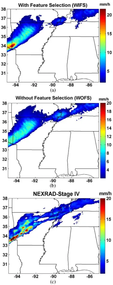
Fig. 2. Estimated hourly rainfall estimates ending at 1000 UTC on Febru-ary 12, 2008. (a) With feature selection. (b) Without feature selection. (c) NEXRAD Stage IV.
If the data is uniformly distributed, the entropy is maximum [6]. When the data is well-formed, the uncertainty is low and the entropy is low [16]. It is expected that the irrelevant and redundant features increase the entropy of the data set [16].
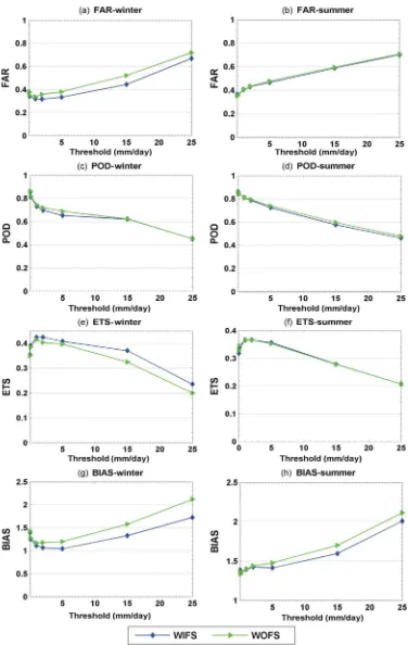
Fig. 3. Validation results for the 2008 winter and summer seasons (daily estimate). (a) and (b) False alarm ratio. (c) and (d) Probability of detection. (e) and (f) Equitable threat score. (g) and (h) Bias.
III. VERIFICATION OFRESULTS
The study region covers 30◦ N to 38◦ N and −95◦ E to −85◦E of the United States. The winter (January and February)
and summer (June, July, and August) periods of 2008 are used for testing. Note that approximately 7300 images of the
The IR brightness temperature observations are obtained from the GOES-12 satellite. Produced by the National Centers for Environmental Prediction, the NEXRAD Stage IV precip-itation products are used for training and validation [13]. The IR data from GOES-12 (Channel 4) has 30-min time interval images that cover the entire area of study. It also has a nominal spatial resolution of 4×4 km2. The spatial resolution for
NEXRAD Stage IV is 4×4 km2, and the data are available
as 1, 6, and 24 hourly accumulated precipitation values over the United States. In this paper, the total features are 62, and by applying the features selection technique, the selected features are reduced to 11. Note that k (the FSS parameter) is set to 20.
Fig. 2 shows an example of the hourly precipitation esti-mate of the two algorithms, with and without feature selection (hereafter they are called with feature selection (WIFS)/without feature selection (WOFS)), at 1000 UTC on February 12, 2008 (the precipitation estimates are typically derived every 30 min; however, for validating the results against NEXRAD Stage IV, we accumulate them in hourly estimates). In addition, the corresponding NEXRAD Stage IV data are shown in Fig. 2(c). Note that this figure corresponds to the results obtained from just one example out of the approximately 7300 images used in this study for testing.
A set of four verification metrics are utilized to evaluate the performance of the algorithms against the daily NEXRAD stage IV product at rainfall thresholds of 0.01, 0.1, 1, 2, 5, 15, and 25 mm/day. These metrics are: probability of detection (POD), false-alarm ratio (FAR), equitable threat score (ETS), and bias [2]. The bias is the ratio of the estimated to observed rain areas. A bias value of 1 indicates that the estimation and observation have identical area coverage [2]. Note that the bias metric is related to hits, false alarms, misses, and correct negatives.
The performance of WIFS and WOFS is shown in Fig. 3 for the winter and summer seasons of 2008 at different rainfall thresholds. Fig. 3(a) and (b) shows the FAR of both algorithms for the winter and summer. The FAR of the WIFS in the winter is less than that of the WOFS at almost all threshold levels. At some threshold levels in the winter, the WIFS provides up to 10% less FAR than the WOFS. In the summer, the two algorithms have the same performance in terms of FAR. Fig. 3(c) and (d) shows the performance of POD for the two algorithms (WIFS and WOFS). Except for a slight decrease in medium rainfall thresholds in the winter, the POD of the WIFS and WOFS are similar. Fig. 3(e) and (f) show the ETS of the two algorithms in the winter and summer. In the winter, the ETS of the WIFS improves at almost all rainfall thresholds, with approximately 7% improvement occurring at medium and high rainfall threshold levels. In the summer, the ETS of the two algorithms are the same at all rainfall thresholds. Fig. 3(g) and (h) shows the bias of both algorithms in the winter and summer. Using feature selection, the bias decreases in both the winter and summer almost at all rainfall thresholds. The bias decreases more in medium and high rainfall thresholds. In the winter, the bias decreases in a range of 0.1 to 0.4, and in the summer, it decreases from 0.1 to 0.2 mm/day.
It is worthy to mention that the ETS improvement in the winter can be related to the type of cloud covers. Different cloud types occur in the summer and winter seasons. From
the results presented, it can be inferred that some features provide irrelevant rain-rate information from some cloud types occurring in the winter. These features are more likely being removed by the feature selection technique. As a result, the ETS improves in the winter.
IV. CONCLUSION
A feature selection technique is applied to the PERSIANN-CCS enriched with wavelet features to enhance rainfall precip-itation estimation. The feature selection technique includes a FSS method and a FFSGA. The EI fitness function is exploited as the feature subset evaluator. The results show that, in the winter season, the WIFS algorithm provides approximately 7% ETS improvement at medium and high rainfall threshold levels compared to the WOFS algorithm. It also decreases the bias in the winter and summer seasons. Furthermore, it greatly reduces the dimensionality from 62 to 11.
ACKNOWLEDGMENT
The authors thank Dr. S. Sorooshian and Dr. K-L. Hsu at UC Irvine for the PERSIANN-CCS data and the helpful discussions.
REFERENCES
[1] E. N. Anagnostou, “Overview of overland satellite rainfall estimation for hydro-meteorological applications,”Surveys Geophys., vol. 25, no. 5/6, pp. 511–537, 2004.
[2] E. E. Ebert, J. E. Janowiak, and C. Kidd, “Comparison of near-real-time precipitation estimates from satellite observations and numerical models,”
Bull. Amer. Meteorol. Soc., vol. 88, no. 1, pp. 47–64, 2007.
[3] H. Liu and L. Yu, “Toward integrating feature selection algorithms for classification and clustering,”IEEE Trans. Knowl. Data Eng., vol. 17, no. 4, pp. 491–502, Apr. 2005.
[4] L. Zhou, L. Wang, and C. Shen, “Feature selection with redundancy-constrained class separability,”IEEE Trans. Neural Netw., vol. 21, no. 5, pp. 853–858, May 2010.
[5] A. P. Estevez, M. Tesmer, A. C. Perez, and M. J. Zurada, “Normalized mutual information feature selection,”IEEE Trans. Neural Netw., vol. 20, no. 2, pp. 189–201, Feb. 2009.
[6] P. Mitra, C. A. Murthy, and S. K. Pal, “Unsupervised feature selection using feature similarity,”IEEE Trans. Pattern Anal. Mach. Intell., vol. 24, no. 3, pp. 301–312, Mar. 2002.
[7] Z. Zhu, Y. Ong, and M. Dash, “Wrapper-filter feature selection algorithm using a memetic framework,”IEEE Trans. Syst., Man, Cybern. B, Cy-bern., vol. 37, no. 1, pp. 70–76, Feb. 2007.
[8] H. Liu and H. Motoda, Computational Methods of Feature Selection. Boca Raton, FL: Chapman & Hall, 2007.
[9] I. Guyon and A. Elisseeff, “An introduction to variable and feature selec-tion,”J. Mach. Learn. Res., vol. 3, pp. 1157–1182, Mar. 2003.
[10] Y. Hong, K. L. Hsu, S. Sorooshian, and X. G. Gao, “Precipitation esti-mation from remotely sensed imagery using an artificial neural network cloud classification system,”J. Appl. Meteorol., vol. 43, no. 12, pp. 1834– 1852, 2004.
[11] M. Mahrooghy, V. G. Anantharaj, N. H. Younan, W. A. Petersen, F. J. Turk, and J. Aanstoos, “Infrared satellite precipitation estimate using waveletbased cloud classification and radar calibration,” inProc. IEEE IGARSS, Honolulu, HI, Jul. 2010, pp. 2345–2348.
[12] T. Kohonen, “Self-organized formation of topologically correct features maps,”Biol. Cybern., vol. 43, no. 1, pp. 59–69, 1982.
[13] Y. Lin and K. E. Mitchell, “The NCEP stage II/IV hourly precipitation analyses: Development and applications,” inProc. 19th Conf. Hydrol., Amer. Meteorol. Soc., San Diego, CA, 2005, 1.2.
[14] J. C. Grzegorz and W. F. Krajewski, “Comments on the window prob-ability matching method for rainfall measurements with radar,”J. Appl. Meteorol., vol. 36, no. 3, pp. 243–246, Mar. 1997.
[15] D. Goldberg,Genetic Algorithms in Search, Optimization, and Machine Learning. Boston, MA: Addison-Wesley, 1989.