Big Data for Chimps
Big Data for Chimps
by Philip Kromer and Russell Jurney
Copyright © 2016 Philip Kromer and Russell Jurney. All rights reserved. Printed in the United States of America.
Published by O’Reilly Media, Inc., 1005 Gravenstein Highway North, Sebastopol, CA 95472. O’Reilly books may be purchased for educational, business, or sales promotional use. Online editions are also available for most titles (http://safaribooksonline.com). For more information, contact our corporate/institutional sales department: 800-998-9938 or [email protected].
Acquisitions Editor: Mike Loukides
Editors: Meghan Blanchette and Amy Jollymore
Production Editor: Matthew Hacker Copyeditor: Jasmine Kwityn
Proofreader: Rachel Monaghan Indexer: Wendy Catalano
Interior Designer: David Futato
Revision History for the First Edition 2015-09-25: First Release
See http://oreilly.com/catalog/errata.csp?isbn=9781491923948 for release details.
The O’Reilly logo is a registered trademark of O’Reilly Media, Inc. Big Data for Chimps, the cover image of a chimpanzee, and related trade dress are trademarks of O’Reilly Media, Inc.
While the publisher and the authors have used good faith efforts to ensure that the information and instructions contained in this work are accurate, the publisher and the authors disclaim all
responsibility for errors or omissions, including without limitation responsibility for damages
resulting from the use of or reliance on this work. Use of the information and instructions contained in this work is at your own risk. If any code samples or other technology this work contains or describes is subject to open source licenses or the intellectual property rights of others, it is your responsibility to ensure that your use thereof complies with such licenses and/or rights.
Preface
Big Data for Chimps will explain a practical, actionable view of big data. This view will be centered on tested best practices as well as give readers street-fighting smarts with Hadoop.
Readers will come away with a useful, conceptual idea of big data. Insight is data in context. The key to understanding big data is scalability: infinite amounts of data can rest upon distinct pivot points. We will teach you how to manipulate data about these pivot points.
What This Book Covers
Big Data for Chimps shows you how to solve important problems in large-scale data processing using simple, fun, and elegant tools.
Finding patterns in massive event streams is an important, hard problem. Most of the time, there aren’t earthquakes — but the patterns that will let you predict one in advance lie within the data from those quiet periods. How do you compare the trillions of subsequences in billions of events, each to each other, to find the very few that matter? Once you have those patterns, how do you react to them in real time?
We’ve chosen case studies anyone can understand, and that are general enough to apply to whatever problems you’re looking to solve. Our goal is to provide you with the following:
The ability to think at scale--equipping you with a deep understanding of how to break a problem into efficient data transformations, and of how data must flow through the cluster to effect those transformations
Detailed example programs applying Hadoop to interesting problems in context Advice and best practices for efficient software development
All of the examples use real data, and describe patterns found in many problem domains, as you: Create statistical summaries
Identify patterns and groups in the data Search, filter, and herd records in bulk
The emphasis on simplicity and fun should make this book especially appealing to beginners, but this is not an approach you’ll outgrow. We’ve found it’s the most powerful and valuable approach for creative analytics. One of our maxims is “robots are cheap, humans are important”: write readable, scalable code now and find out later whether you want a smaller cluster. The code you see is adapted from programs we write at Infochimps and Data Syndrome to solve enterprise-scale business
problems, and these simple high-level transformations meet our needs.
Who This Book Is For
We’d like for you to be familiar with at least one programming language, but it doesn’t have to be Python or Pig. Familiarity with SQL will help a bit, but isn’t essential. Some exposure to working with data in a business intelligence or analysis background will be helpful.
Who This Book Is Not For
This is not Hadoop: The Definitive Guide (that’s already been written, and well); this is more like
Hadoop: A Highly Opinionated Guide. The only coverage of how to use the bare Hadoop API is to say, “in most cases, don’t.” We recommend storing your data in one of several highly
space-inefficient formats and in many other ways encourage you to willingly trade a small performance hit for a large increase in programmer joy. The book has a relentless emphasis on writing scalable code, but no content on writing performant code beyond the advice that the best path to a 2x speedup is to launch twice as many machines.
That is because for almost everyone, the cost of the cluster is far less than the opportunity cost of the data scientists using it. If you have not just big data but huge data (let’s say somewhere north of 100 terabytes), then you will need to make different trade-offs for jobs that you expect to run repeatedly in production. However, even at petabyte scale, you will still develop in the manner we outline.
The book does include some information on provisioning and deploying Hadoop, and on a few
What This Book Does Not Cover
We are not currently planning to cover Hive. The Pig scripts will translate naturally for folks who are already familiar with it.
This book picks up where the Internet leaves off. We’re not going to spend any real time on
information well covered by basic tutorials and core documentation. Other things we do not plan to include:
Installing or maintaining Hadoop.
Other MapReduce-like platforms (Disco, Spark, etc.) or other frameworks (Wukong, Scalding, Cascading).
At a few points, we’ll use Unix text utils (cut/wc/etc.), but only as tools for an immediate
Theory: Chimpanzee and Elephant
Practice: Hadoop
In Doug Cutting’s words, Hadoop is the “kernel of the big-data operating system.” It is the dominant batch-processing solution, has both commercial enterprise support and a huge open source
community, and runs on every platform and cloud — and there are no signs any of that will change in the near term.
The code in this book will run unmodified on your laptop computer or on an industrial-strength
Example Code
You can check out the source code for the book using Git:
git clone https://github.com/bd4c/big_data_for_chimps-code
A Note on Python and MrJob
Helpful Reading
Programming Pig by Alan Gates is a more comprehensive introduction to the Pig Latin language and Pig tools. It is highly recommended.
Hadoop: The Definitive Guide by Tom White is a must-have. Don’t try to absorb it whole — the most powerful parts of Hadoop are its simplest parts — but you’ll refer to it often as your applications reach production.
Feedback
Contact us! If you have questions, comments, or complaints, the issue tracker is the best forum for sharing those. If you’d like something more direct, email [email protected] and
[email protected] (your eager authors) — and you can feel free to cc: [email protected]
(our ever-patient editor). We’re also available via Twitter: Flip Kromer (@mrflip)
Conventions Used in This Book
The following typographical conventions are used in this book:
Italic
Indicates new terms, URLs, email addresses, filenames, and file extensions.
Constant width
Used for program listings, as well as within paragraphs to refer to program elements such as variable or function names, databases, datatypes, environment variables, statements, and keywords.
Constant width bold
Shows commands or other text that should be typed literally by the user.
Constant width italic
Shows text that should be replaced with user-supplied values or by values determined by context.
TIP This element signifies a tip or suggestion.
NOTE This element signifies a general note.
WARNING
Using Code Examples
Supplemental material (code examples, exercises, etc.) is available for download at https://github.com/bd4c/big_data_for_chimps-code.
This book is here to help you get your job done. In general, if example code is offered with this book, you may use it in your programs and documentation. You do not need to contact us for permission unless you’re reproducing a significant portion of the code. For example, writing a program that uses several chunks of code from this book does not require permission. Selling or distributing a CD-ROM of examples from O’Reilly books does require permission. Answering a question by citing this book and quoting example code does not require permission. Incorporating a significant amount of example code from this book into your product’s documentation does require permission.
We appreciate, but do not require, attribution. An attribution usually includes the title, author, publisher, and ISBN. For example: “Big Data for Chimps by Philip Kromer and Russell Jurney (O’Reilly). Copyright 2015 Philip Kromer and Russell Jurney, 978-1-491-92394-8.”
Safari® Books Online
NOTE
Safari Books Online is an on-demand digital library that delivers expert content in both book and video form from the world’s leading authors in technology and business.
Technology professionals, software developers, web designers, and business and creative professionals use Safari Books Online as their primary resource for research, problem solving, learning, and certification training.
Safari Books Online offers a range of plans and pricing for enterprise, government, education, and individuals.
How to Contact Us
Please address comments and questions concerning this book to the publisher: O’Reilly Media, Inc.
1005 Gravenstein Highway North Sebastopol, CA 95472
800-998-9938 (in the United States or Canada) 707-829-0515 (international or local)
707-829-0104 (fax)
We have a web page for this book, where we list errata, examples, and any additional information. You can access this page at http://bit.ly/big_data_4_chimps.
To comment or ask technical questions about this book, send email to [email protected]. For more information about our books, courses, conferences, and news, see our website at
http://www.oreilly.com.
Find us on Facebook: http://facebook.com/oreilly Follow us on Twitter: http://twitter.com/oreillymedia
Part I. Introduction: Theory and Tools
In Chapters 1–4, we’ll introduce you to the basics about Hadoop and MapReduce, and to the tools you’ll be using to process data at scale using Hadoop.
We’ll start with an introduction to Hadoop and MapReduce, and then we’ll dive into MapReduce and explain how it works. Next, we’ll introduce you to our primary dataset: baseball statistics. Finally, we’ll introduce you to Apache Pig, the tool we use to process data in the rest of the book.
Chapter 1. Hadoop Basics
Hadoop is a large and complex beast. It can be bewildering to even begin to use the system, and so in this chapter we’re going to purposefully charge through the minimum requirements for getting started with launching jobs and managing data. In this book, we will try to keep things as simple as possible. For every one of Hadoop’s many modes, options, and configurations that is essential, there are many more that are distracting or even dangerous. The most important optimizations you can make come from designing efficient workflows, and even more so from knowing when to spend highly valuable programmer time to reduce compute time.
In this chapter, we will equip you with two things: the necessary mechanics of working with Hadoop, and a physical intuition for how data and computation move around the cluster during a job.
The key to mastering Hadoop is an intuitive, physical understanding of how data moves around a Hadoop cluster. Shipping data from one machine to another — even from one location on disk to another — is outrageously costly, and in the vast majority of cases, dominates the cost of your job. We’ll describe at a high level how Hadoop organizes data and assigns tasks across compute nodes so that as little data as possible is set in motion; we’ll accomplish this by telling a story that features a physical analogy and by following an example job through its full lifecycle. More importantly, we’ll show you how to read a job’s Hadoop dashboard to understand how much it cost and why. Your goal for this chapter is to take away a basic understanding of how Hadoop distributes tasks and data, and the ability to run a job and see what’s going on with it. As you run more and more jobs through the remaining course of the book, it is the latter ability that will cement your intuition.
What does Hadoop do, and why should we learn about it? Hadoop enables the storage and processing of large amounts of data. Indeed, it is Apache Hadoop that stands at the middle of the big data trend. The Hadoop Distributed File System (HDFS) is the platform that enabled cheap storage of vast
amounts of data (up to petabytes and beyond) using affordable, commodity machines. Before Hadoop, there simply wasn’t a place to store terabytes and petabytes of data in a way that it could be easily accessed for processing. Hadoop changed everything.
Chimpanzee and Elephant Start a Business
A few years back, two friends — JT, a gruff chimpanzee, and Nanette, a meticulous matriarch elephant — decided to start a business. As you know, chimpanzees love nothing more than sitting at keyboards processing and generating text. Elephants have a prodigious ability to store and recall information, and will carry huge amounts of cargo with great determination. This combination of skills impressed a local publishing company enough to earn their first contract, so Chimpanzee and Elephant, Incorporated (C&E for short) was born.
The publishing firm’s project was to translate the works of Shakespeare into every language known to man, so JT and Nanette devised the following scheme. Their crew set up a large number of cubicles, each with one elephant-sized desk and several chimp-sized desks, and a command center where JT and Nanette could coordinate the action.
As with any high-scale system, each member of the team has a single responsibility to perform. The task of each chimpanzee is simply to read a set of passages and type out the corresponding text in a new language. JT, their foreman, efficiently assigns passages to chimpanzees, deals with absentee workers and sick days, and reports progress back to the customer. The task of each librarian elephant is to maintain a neat set of scrolls, holding either a passage to translate or some passage’s translated result. Nanette serves as chief librarian. She keeps a card catalog listing, for every book, the location and essential characteristics of the various scrolls that maintain its contents.
When workers clock in for the day, they check with JT, who hands off the day’s translation manual and the name of a passage to translate. Throughout the day, the chimps radio progress reports in to JT; if their assigned passage is complete, JT will specify the next passage to translate.
If you were to walk by a cubicle mid-workday, you would see a highly efficient interplay between chimpanzee and elephant, ensuring the expert translators rarely had a wasted moment. As soon as JT radios back what passage to translate next, the elephant hands it across. The chimpanzee types up the translation on a new scroll, hands it back to its librarian partner, and radios for the next passage. The librarian runs the scroll through a fax machine to send it to two of its counterparts at other cubicles, producing the redundant, triplicate copies Nanette’s scheme requires.
The librarians in turn notify Nanette which copies of which translations they hold, which helps Nanette maintain her card catalog. Whenever a customer comes calling for a translated passage, Nanette fetches all three copies and ensures they are consistent. This way, the work of each monkey can be compared to ensure its integrity, and documents can still be retrieved even if a cubicle radio fails.
Map-Only Jobs: Process Records Individually
As you’d guess, the way Chimpanzee and Elephant organize their files and workflow corresponds directly with how Hadoop handles data and computation under the hood. We can now use it to walk you through an example in detail.
The bags on trees scheme represents transactional relational database systems. These are often the systems that Hadoop data processing can augment or replace. The “NoSQL” (Not Only SQL)
movement of which Hadoop is a part is about going beyond the relational database as a one-size-fits-all tool, and using different distributed systems that better suit a given problem.
Nanette is the Hadoop NameNode. The NameNode manages the HDFS. It stores the directory tree structure of the filesystem (the card catalog), and references to the data nodes for each file (the librarians). You’ll note that Nanette worked with data stored in triplicate. Data on HDFS is
duplicated three times to ensure reliability. In a large enough system (thousands of nodes in a petabyte Hadoop cluster), individual nodes fail every day. In that case, HDFS automatically creates a new duplicate for all the files that were on the failed node.
JT is the JobTracker. He coordinates the work of individual MapReduce tasks into a cohesive system. The JobTracker is responsible for launching and monitoring the individual tasks of a
MapReduce job, which run on the nodes that contain the data a particular job reads. MapReduce jobs are divided into a map phase, in which data is read, and a reduce phase, in which data is aggregated by key and processed again. For now, we’ll cover map-only jobs (we’ll introduce reduce in
Chapter 2).
Note that in YARN (Hadoop 2.0), the terminology changed. The JobTracker is called the
Pig Latin Map-Only Job
To illustrate how Hadoop works, let’s dive into some code with the simplest example possible. We may not be as clever as JT’s multilingual chimpanzees, but even we can translate text into a language we’ll call Igpay Atinlay.2 For the unfamiliar, here’s how to translate standard English into Igpay
Atinlay:
If the word begins with a consonant-sounding letter or letters, move them to the end of the word and then add “ay”: “happy” becomes “appy-hay,” “chimp” becomes “imp-chay,” and “yes” becomes “es-yay.”
In words that begin with a vowel, just append the syllable “way”: “another” becomes “another-way,” “elephant” becomes “elephant-way.”
Example 1-1 is our first Hadoop job, a program that translates plain-text files into Igpay Atinlay. This is a Hadoop job stripped to its barest minimum, one that does just enough to each record that you believe it happened but with no distractions. That makes it convenient to learn how to launch a job, how to follow its progress, and where Hadoop reports performance metrics (e.g., for runtime and amount of data moved). What’s more, the very fact that it’s trivial makes it one of the most important examples to run. For comparable input and output size, no regular Hadoop job can outperform this one in practice, so it’s a key reference point to carry in mind.
We’ve written this example in Python, a language that has become the lingua franca of data science. You can run it over a text file from the command line — or run it over petabytes on a cluster (should you for whatever reason have a petabyte of text crying out for pig-latinizing).
Example 1-1. Igpay Atinlay translator, pseudocode
for each line,
recognize each word in the line and change it as follows:
separate the head consonants (if any) from the tail of the word if there were no initial consonants, use 'w' as the head
give the tail the same capitalization as the word thus changing the word to "tail-head-ay"
end
having changed all the words, emit the latinized version of the line end
original_word = ''.join(word) head, tail = word
head = 'w' if not head else head pig_latin_word = tail + head + 'ay' if CAPITAL_RE.match(pig_latin_word):
else:
pig_latin_word = pig_latin_word.lower() pig_latin_words.append(pig_latin_word) return " ".join(pig_latin_words)
if __name__ == '__main__': for line in sys.stdin: print mapper(line)
It’s best to begin developing jobs locally on a subset of data, because they are faster and cheaper to run. To run the Python script locally, enter this into your terminal’s command line:
cat /data/gold/text/gift_of_the_magi.txt|python examples/ch_01/pig_latin.py
The output should look like this:
Theway agimay asway youway owknay ereway iseway enmay onderfullyway iseway enmay owhay oughtbray iftsgay otay ethay Babeway inway ethay angermay Theyway
inventedway ethay artway ofway ivinggay Christmasway esentspray Beingway iseway eirthay iftsgay ereway onay oubtday iseway onesway ossiblypay earingbay ethay ivilegepray ofway exchangeway inway asecay ofway uplicationday Andway erehay Iway avehay amelylay elatedray otay youway ethay uneventfulway oniclechray ofway otway oolishfay ildrenchay inway away atflay owhay ostmay unwiselyway
acrificedsay orfay eachway otherway ethay eatestgray easurestray ofway eirthay ousehay Butway inway away astlay ordway otay ethay iseway ofway esethay aysday etlay itway ebay aidsay atthay ofway allway owhay ivegay iftsgay esethay otway ereway ethay isestway Ofway allway owhay ivegay andway eceiveray iftsgay uchsay asway eythay areway isestway Everywhereway eythay areway isestway Theyway areway ethay agimay
That’s what it looks like when run locally. Let’s run it on a real Hadoop cluster to see how it works when an elephant is in charge.
NOTE
Setting Up a Docker Hadoop Cluster
We’ve prepared a docker image you can use to create a Hadoop environment with Pig and Python already installed, and with the example data already mounted on a drive. You can begin by checking out the code. If you aren’t familiar with Git, check out the Git home page and install it. Then proceed to clone the example code Git repository, which includes the docker setup:
git clone --recursive http://github.com/bd4c/big_data_for_chimps-code.git \ bd4c-code
cd bd4c-code ls
You should see:
Gemfile README.md cluster docker examples junk notes numbers10k.txt vendor
Now you will need to install VirtualBox for your platform, which you can download from the
VirtualBox website. Next, you will need to install Boot2Docker, which you can find from
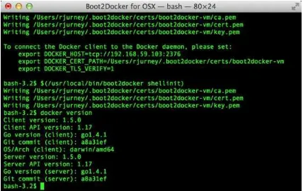
https://docs.docker.com/installation/. Run Boot2Docker from your OS menu, which (on OS X or Linux) will bring up a shell, as shown in Figure 1-1.
Figure 1-1. Boot2Docker for OS X
We use Ruby scripts to set up our docker environment, so you will need Ruby v. >1.9.2 or >2.0. Returning to your original command prompt, from inside the bd4c-code directory, let’s install the
Ruby libraries needed to set up our docker images:
Next, change into the cluster directory, and repeat bundle install:
cd cluster bundle install
You can now run docker commands against this VirtualBox virtual machine (VM) running the docker daemon. Let’s start by setting up port forwarding from localhost to our docker VM. From the cluster
directory:
boot2docker down
bundle exec rake docker:open_ports
While we have the docker VM down, we’re going to need to make an adjustment in VirtualBox. We need to increase the amount of RAM given to the VM to at least 4 GB. Run VirtualBox from your OS’s GUI, and you should see something like Figure 1-2.
Figure 1-2. Boot2Docker VM inside VirtualBox
Select the Boot2Docker VM, and then click Settings. As shown in Figure 1-3, you should now select the System tab, and adjust the RAM slider right until it reads at least 4096 MB. Click OK.
Now you can close VirtualBox, and bring Boot2Docker back up:
boot2docker up
This command will print something like the following:
Writing /Users/rjurney/.boot2docker/certs/boot2docker-vm/ca.pem Writing /Users/rjurney/.boot2docker/certs/boot2docker-vm/cert.pem Writing /Users/rjurney/.boot2docker/certs/boot2docker-vm/key.pem export DOCKER_TLS_VERIFY=1
export DOCKER_HOST=tcp://192.168.59.103:2376
export DOCKER_CERT_PATH=/Users/rjurney/.boot2docker/certs/boot2docker-vm
Figure 1-3. VirtualBox interface
Now is a good time to put these lines in your ~/.bashrc file (make sure to substitute your home
directory for <home_directory>):
export DOCKER_TLS_VERIFY=1 export DOCKER_IP=192.168.59.103
export DOCKER_HOST=tcp://$DOCKER_IP:2376
export DOCKER_CERT_PATH=/<home_directory>/.boot2docker/certs/boot2docker-vm
You can achieve that, and update your current environment, via:
echo 'export DOCKER_TLS_VERIFY=1' >> ~/.bashrc echo 'export DOCKER_IP=192.168.59.103' >> ~/.bashrc
echo 'export DOCKER_HOST=tcp://$DOCKER_IP:2376' >> ~/.bashrc
echo 'export DOCKER_CERT_PATH=/<home_dir>/.boot2docker/certs/boot2docker-vm' \ >> ~/.bashrc
Check that these environment variables are set, and that the docker client can connect, via:
echo $DOCKER_IP echo $DOCKER_HOST bundle exec rake ps
Now you’re ready to set up the docker images. This can take a while, so brew a cup of tea after running:
bundle exec rake images:pull
Once that’s done, you should see:
Status: Image is up to date for blalor/docker-hosts:latest
Now we need to do some minor setup on the Boot2Docker virtual machine. Change terminals to the Boot2Docker window, or from another shell run boot2docker ssh, and run these commands:
mkdir -p /tmp/bulk/hadoop # view all logs there # so that docker-hosts can make container hostnames resolvable sudo touch /var/lib/docker/hosts
sudo chmod 0644 /var/lib/docker/hosts sudo chown nobody /var/lib/docker/hosts exit
Now exit the Boot2Docker shell.
Back in the cluster directory, it is time to start the cluster helpers, which set up hostnames among
the containers:
bundle exec rake helpers:run
If everything worked, you can now run cat /var/lib/docker/hosts on the Boot2Docker host, and
it should be filled with information. Running bundle exec rake ps should show containers for host_filer and nothing else.
Next, let’s set up our example data. Run the following:
bundle exec rake data:create show_output=true
At this point, you can run bundle exec rake ps and you should see five containers, all stopped.
Start these containers using:
bundle exec rake hadoop:run
This will start the Hadoop containers. You can stop/start them with:
Now ssh to your new Hadoop cluster:
ssh -i insecure_key.pem chimpy@$DOCKER_IP -p 9022 # Password chimpy
You can see that the example data is available on the local filesystem:
chimpy@lounge:~$ ls /data/gold/
airline_flights/ demographic/ geo/ graph/ helpers/ serverlogs/ sports/ text/ twitter/ wikipedia/ CREDITS.md README-archiver.md README.md
Now you can run Pig, in local mode:
pig -l /tmp -x local
Run the Job
First, let’s test on the same tiny little file we used before. The following command does not process any data but instead instructs Hadoop to process the data. The command will generate output that contains information about how the job is progressing:
hadoop jar /usr/lib/hadoop-mapreduce/hadoop-streaming.jar \
-Dmapreduce.cluster.local.dir=/home/chimpy/code -fs local -jt local \ -file ./examples/ch_01/pig_latin.py -mapper ./examples/ch_01/pig_latin.py \ -input /data/gold/text/gift_of_the_magi.txt -output ./translation.out
You should see something like this:
WARN fs.FileSystem: "local" is a deprecated filesystem name. Use "file:///"... WARN streaming.StreamJob: -file option is deprecated, please use generic... packageJobJar: [./examples/ch_01/pig_latin.py] [] /tmp/...
INFO Configuration.deprecation: session.id is deprecated. Instead, use... INFO jvm.JvmMetrics: Initializing JVM Metrics with processName=JobTracker... INFO jvm.JvmMetrics: Cannot initialize JVM Metrics with...
INFO mapred.FileInputFormat: Total input paths to process : 1 INFO mapreduce.JobSubmitter: number of splits:1
INFO mapreduce.JobSubmitter: Submitting tokens for job: job_local292160259_0001 WARN conf.Configuration: file:/tmp/hadoop-chimpy/mapred/staging/...
WARN conf.Configuration: file:/tmp/hadoop-chimpy/mapred/staging/... INFO mapred.LocalDistributedCacheManager: Localized file:/home/chimpy/... WARN conf.Configuration: file:/home/chimpy/code/localRunner/chimpy/... WARN conf.Configuration: file:/home/chimpy/code/localRunner/chimpy/... INFO mapreduce.Job: The url to track the job: http://localhost:8080/ INFO mapred.LocalJobRunner: OutputCommitter set in config null INFO mapreduce.Job: Running job: job_local292160259_0001 INFO mapred.LocalJobRunner: OutputCommitter is...
INFO mapred.LocalJobRunner: Waiting for map tasks INFO mapred.LocalJobRunner: Starting task:...
INFO mapred.Task: Using ResourceCalculatorProcessTree : [ ] INFO mapred.MapTask: Processing split: file:/data/gold/text/... INFO mapred.MapTask: numReduceTasks: 1
INFO mapred.MapTask: (EQUATOR) 0 kvi 26214396(104857584) INFO mapred.MapTask: mapreduce.task.io.sort.mb: 100 INFO mapred.MapTask: soft limit at 83886080
INFO mapred.MapTask: bufstart = 0; bufvoid = 104857600 INFO mapred.MapTask: kvstart = 26214396; length = 6553600 INFO mapred.MapTask: Map output collector class =...
INFO streaming.PipeMapRed: PipeMapRed exec [/home/chimpy/code/./pig_latin.py] INFO streaming.PipeMapRed: R/W/S=1/0/0 in:NA [rec/s] out:NA [rec/s]
INFO streaming.PipeMapRed: R/W/S=10/0/0 in:NA [rec/s] out:NA [rec/s] INFO streaming.PipeMapRed: R/W/S=100/0/0 in:NA [rec/s] out:NA [rec/s] INFO streaming.PipeMapRed: Records R/W=225/1
INFO streaming.PipeMapRed: MRErrorThread done INFO streaming.PipeMapRed: mapRedFinished INFO mapred.LocalJobRunner:
INFO mapred.MapTask: Starting flush of map output INFO mapred.MapTask: Spilling map output
INFO mapred.MapTask: bufstart = 0; bufend = 16039; bufvoid = 104857600 INFO mapred.MapTask: kvstart = 26214396(104857584); kvend =...
INFO mapred.MapTask: Finished spill 0
INFO mapred.Task: Task:attempt_local292160259_0001_m_000000_0 is done. And is... INFO mapred.LocalJobRunner: Records R/W=225/1
INFO mapreduce.Job: Job job_local292160259_0001 running in uber mode : false INFO mapreduce.Job: map 100% reduce 0%
INFO reduce.MergeManagerImpl: MergerManager: memoryLimit=652528832... INFO reduce.EventFetcher: attempt_local292160259_0001_r_000000_0 Thread... INFO reduce.LocalFetcher: localfetcher#1 about to shuffle output of map... INFO reduce.InMemoryMapOutput: Read 16491 bytes from map-output for...
INFO reduce.MergeManagerImpl: closeInMemoryFile -> map-output of size: 16491... INFO reduce.EventFetcher: EventFetcher is interrupted.. Returning
INFO mapred.LocalJobRunner: 1 / 1 copied.
INFO reduce.MergeManagerImpl: finalMerge called with 1 in-memory map-outputs... INFO mapred.Merger: Merging 1 sorted segments
INFO mapred.Merger: Down to the last merge-pass, with 1 segments left of... INFO reduce.MergeManagerImpl: Merged 1 segments, 16491 bytes to disk to... INFO reduce.MergeManagerImpl: Merging 1 files, 16495 bytes from disk
INFO reduce.MergeManagerImpl: Merging 0 segments, 0 bytes from memory into... INFO mapred.Merger: Merging 1 sorted segments
INFO mapred.Merger: Down to the last merge-pass, with 1 segments left of... INFO mapred.LocalJobRunner: 1 / 1 copied.
INFO mapred.Task: Task:attempt_local292160259_0001_r_000000_0 is done. And is... INFO mapred.LocalJobRunner: 1 / 1 copied.
INFO mapred.Task: Task attempt_local292160259_0001_r_000000_0 is allowed to... INFO output.FileOutputCommitter: Saved output of task...
INFO mapred.LocalJobRunner: reduce > reduce
INFO mapred.Task: Task 'attempt_local292160259_0001_r_000000_0' done. INFO mapred.LocalJobRunner: Finishing task:...
INFO mapred.LocalJobRunner: reduce task executor complete. INFO mapreduce.Job: map 100% reduce 100%
INFO mapreduce.Job: Job job_local292160259_0001 completed successfully INFO mapreduce.Job: Counters: 33
File System Counters
FILE: Number of bytes read=58158 FILE: Number of bytes written=581912 FILE: Number of read operations=0 FILE: Number of large read operations=0 FILE: Number of write operations=0 Map-Reduce Framework
Map input records=225 Map output records=225 Map output bytes=16039
Map output materialized bytes=16495 Input split bytes=93
Combine input records=0 Combine output records=0 Reduce input groups=180 Reduce shuffle bytes=16495 Reduce input records=225 Reduce output records=225 Spilled Records=450
Physical memory (bytes) snapshot=0 Virtual memory (bytes) snapshot=0
Wrapping Up
In this chapter, we’ve equipped you with two things: the necessary mechanics of working with
Hadoop, and a physical intuition for how data and computation move around the cluster during a job. We started with a story about JT and Nanette, and learned about the Hadoop JobTracker, NameNode, and filesystem. We proceeded with a Pig Latin example, and ran it on a real Hadoop cluster.
We’ve covered the mechanics of the Hadoop Distributed File System (HDFS) and the map-only
portion of MapReduce, and we’ve set up a virtual Hadoop cluster and run a single job on it. Although we are just beginning, we’re already in good shape to learn more about Hadoop.
In the next chapter, you’ll learn about MapReduce jobs — the full power of Hadoop’s processing paradigm. We’ll start by continuing the story of JT and Nannette, and learning more about their next client.
1 Some chimpanzee philosophers have put forth the fanciful conceit of a “paperless” office, requiring impossibilities like a sea of electrons that do the work of a chimpanzee, and disks of magnetized iron that would serve as scrolls. These ideas are, of course, pure lunacy!
Chapter 2. MapReduce
In this chapter, we’re going to build on what we learned about HDFS and the map-only portion of MapReduce and introduce a full MapReduce job and its mechanics. This time, we’ll include both the shuffle/sort phase and the reduce phase. Once again, we begin with a physical metaphor in the form of a story. After that, we’ll walk you through building our first full-blown MapReduce job in Python. At the end of this chapter, you should have an intuitive understanding of how MapReduce works,
including its map, shuffle/sort, and reduce phases.
Chimpanzee and Elephant Save Christmas
Trouble in Toyland
As you know, each year children from every corner of the earth write to Santa to request toys, and Santa — knowing who’s been naughty and who’s been nice — strives to meet the wishes of every good little boy and girl who writes him. He employs a regular army of toymaker elves, each of whom specializes in certain kinds of toys: some elves make action figures and dolls, while others make xylophones and yo-yos (see Figure 2-1).
Figure 2-1. The elves’ workbenches are meticulous and neat
Under the elves’ old system, as bags of mail arrived, they were examined by an elven postal clerk and then hung from the branches of the Big Tree at the center of the Santaplex. Letters were organized on the tree according to the child’s town, as the shipping department has a critical need to organize toys by their final delivery schedule. But the toymaker elves must know what toys to make as well, and so for each letter, a postal clerk recorded its Big Tree coordinates in a ledger that was organized by type of toy.
So to retrieve a letter, a doll-making elf would look under “Doll” in the ledger to find the next letter’s coordinates, then wait as teamster elves swung a big claw arm to retrieve it from the Big Tree (see
Figure 2-2. Little boys’ and girls’ mail is less so
What’s worse, the size of Santa’s operation meant that the workbenches were very far from where letters came in. The hallways were clogged with frazzled elves running from Big Tree to workbench and back, spending as much effort requesting and retrieving letters as they did making toys. This complex transactional system was a bottleneck in toy making, and mechanic elves were constantly scheming ways to make the claw arm cope with increased load. “Throughput, not latency!” trumpeted Nanette. “For hauling heavy loads, you need a stately elephant parade, not a swarm of frazzled
Chimpanzees Process Letters into Labeled Toy Forms
In marched Chimpanzee and Elephant, Inc. JT and Nanette set up a finite number of chimpanzees at a finite number of typewriters, each with an elephant deskmate. Strangely, the C&E solution to the too-many-letters problem involved producing more paper. The problem wasn’t in the amount of paper, it was in all the work being done to service the paper. In the new world, all the rules for handling documents are simple, uniform, and local.
Postal clerks still stored each letter on the Big Tree (allowing the legacy shipping system to continue unchanged), but now also handed off bags holding copies of the mail. As she did with the translation passages, Nanette distributed these mailbags across the desks just as they arrived. The overhead of recording each letter in the much-hated ledger was no more, and the hallways were no longer clogged with elves racing to and fro.
The chimps’ job was to take letters one after another from a mailbag, and fill out a toy form for each request. A toy form has a prominent label showing the type of toy, and a body with all the information you’d expect: name, nice/naughty status, location, and so forth. You can see some examples here:
Deer SANTA
I wood like a doll for me and and an optimus prime robot for my brother joe
I have been good this year love julia
# Good kids, generates a toy for Julia and a toy for her brother # Toy Forms:
# doll | type="green hair" recipient="Joe's sister Julia" # robot | type="optimus prime" recipient="Joe"
Greetings to you Mr Claus, I came to know of you in my search for a reliable and reputable person to handle a very confidential business transaction, which involves the transfer of a large sum of money...
# Spam
# (no toy forms)
HEY SANTA I WANT A YANKEES HAT AND NOT ANY DUMB BOOKS THIS YEAR
FRANK
# Frank is a jerk. He will get a lump of coal. # Toy Forms:
# coal | type="anthracite" recipient="Frank" reason="doesn't like to read"
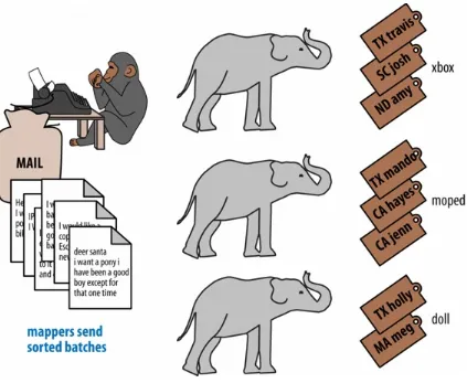
Figure 2-3. A chimp mapping letters
Processing letters in this way represents the map phase of a MapReduce job. The work performed in a map phase could be anything: translation, letter processing, or any other operation. For each record read in the map phase, a mapper can produce zero, one, or more records. In this case, each letter produces one or more toy forms (Figure 2-4). This elf-driven letter operation turns unstructured data (a letter) into a structured record (toy form).
Figure 2-4. A chimp “mapping” letters, producing toy forms
Pygmy Elephants Carry Each Toy Form to the Appropriate
Workbench
Here’s the new wrinkle on top of the system used in the translation project. Next to every desk now stood a line of pygmy elephants, each dressed in a cape listing the types of toy it would deliver. Each desk had a pygmy elephant for archery kits and dolls, another one for xylophones and yo-yos, and so forth — matching the different specialties of toymaker elves.
As the chimpanzees would work through a mailbag, they’d place each toy form into the basket on the back of the pygmy elephant that matched its type. At the completion of a bag (a map phase), the current line of elephants would shuffle off to the workbenches, and behind them a new line of elephants would trundle into place. What fun! (See Figure 2-5.)
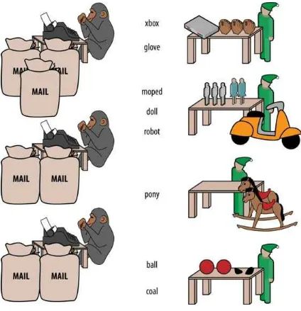
Figure 2-5. The MapReduce shuffle
Finally, the pygmy elephants would march through the now-quiet hallways to the toy shop floor, each reporting to the workbench that matched its toy types. All of the workbenches (the archery kit/doll workbench, the xylophone/yo-yo workbench, etc.) had a line of pygmy elephants, one for every C&E desk.
This activity by the pygmy elephants represents the shuffle/sort phase of a MapReduce job, in which records produced by mappers are grouped by their key (the toy type) and delivered to a reducer for that key (an elf!).
constrained by the overhead of walking the hallway and waiting for Big Tree retrieval on every toy (Figure 2-6).
Figure 2-6. The Reduce process
Our MapReduce job is complete, and toy making is back on track!
Having previously introduced map-only Hadoop in our first story, in this story we introduced the shuffle/sort and reduce operations of Hadoop MapReduce. The toymaker elves are the reducers — they receive all the mapped records (toy forms) corresponding to one or more group keys (the type of toy). The act of toy making is the reduce operation. The pygmy elephants represent the shuffle/sort — the movement of data from mappers to reducers. That is how the MapReduce paradigm works! This simple abstraction powers Hadoop MapReduce programs. It is the simplicity of the scheme that makes it so powerful.
In Chapter 1, you worked with a simple-as-possible Python script, which let you learn the mechanics of running Hadoop jobs and understand the essentials of the HDFS. Document translation is an
Part II.
Hadoop’s real power comes from the ability to process data in context, using what’s known as the MapReduce paradigm. Every MapReduce job is a program with the same three phases: map,
shuffle/sort phase, and reduce. In the map phase, your program processes its input in any way you see fit, emitting labeled output records. Between map and reduce is the Hadoop shuffle/sort. In the
shuffle/sort phase, Hadoop groups and sorts the mapped records according to their labels. Finally, in the reduce phase, your program processes each sorted, labeled group and Hadoop stores its output on HDFS. That shuffle, or grouping-by-label, part is where the magic lies: it ensures that no matter where the relevant records started, they arrive at the same place at a reducer in a predictable manner, ready to be synthesized.
Example: Reindeer Games
Santa Claus and his elves are busy year-round, but Santa’s flying reindeer do not have many
UFO Data
The UFO data is located on the docker HDFS we set up in Chapter 1. Let’s begin by checking our input data. First, ssh into the gateway node and run this command to see the top five lines of the UFO
sightings sample:
cat /data/gold/geo/ufo_sightings/ufo_sightings-sample.tsv|head -5
Note that gold in this path stands for gold standard data (in other words, data that has been checked
and validated to be correct).
The UFO data is in tab-separated values (TSV) format. It has been formatted to fit on the page:
1995-10-09T05:00:00Z 1995-10-09T05:00:00Z Iowa City, IA Man repts. witnessing "flash, ...
1995-10-10T05:00:00Z 1995-10-11T05:00:00Z Milwaukee, WI 2 min. Man on Hwy 43 SW of Mil...
1995-01-01T06:00:00Z 1995-01-03T06:00:00Z Shelton, WA Telephoned Report:CA woman visit...
1995-05-10T05:00:00Z 1995-05-10T05:00:00Z Columbia, MO 2 min. Man repts. son's bizarre...
Group the UFO Sightings by Reporting Delay
In the Chimpanzee and Elephant, Inc., world, a chimp performs the following tasks: 1. Read and understand each letter.
2. Create a new intermediate item having a label (the type of toy, a key) and information about the toy (the work order, a value).
3. Hand it to the elephant who delivers to that toy’s workbench.
We’re going to write a Hadoop mapper that serves a similar purpose: 1. Read the raw data and parse it into a structured record.
2. Create a new intermediate item having a label (the number of days passed before reporting a UFO, a key) and a count (one sighting for each input record, a value).
Mapper
In order to calculate the time delay in reporting UFOs, we’ve got to determine that delay by
subtracting the time the UFO was sighted from the time the UFO was reported. As just outlined, this occurs in the map phase of our MapReduce job. The mapper emits the time delay in days, and a counter (which is always 1).
You may need to install the iso8601 library, via:
pip install iso8601
The mapper code in Python looks like this:
#!/usr/bin/python
# Example MapReduce job: count ufo sightings by location.
import sys, re, time, iso8601 # You can get iso8601 from https://pypi.python.org/ pypi/iso8601
# Pull out city/state from ex: Town, ST word_finder = re.compile("([\w\s]+),\s(\w+)") # Loop through each line from standard input for line in sys.stdin:
# Remove the carriage return, and split on tabs - maximum of 3 fields fields = line.rstrip("\n").split("\t", 2)
try:
# Parse the two dates, then find the time between them sighted_at, reported_at, rest = fields
sighted_dt = iso8601.parse_date(sighted_at) reported_dt = iso8601.parse_date(reported_at) diff = reported_dt - sighted_dt
except:
sys.stderr.write("Bad line: {}".format(line)) continue
# Emit the number of days and one print "\t".join((str(diff.days), "1"))
You can test the mapper like this:
cat /data/gold/geo/ufo_sightings/ufo_sightings-sample.tsv | python \
Reducer
In our previous example, the elf at each workbench saw a series of work orders, with the guarantee that (a) work orders for each toy type are delivered together and in order; and (b) this was the only workbench to receive work orders for that toy type. Similarly, in this job, the reducer receives a series of records (UFO reports, values), grouped by label (the number of days passed before reporting a UFO, a key), with a guarantee that it is the unique processor for such records.
Our reducer is tasked with creating a histogram. The reducer is thus concerned with grouping similar time delays together. The reduce key in this case is the number of days passed before reporting a UFO (e.g., 0, 1, 10, or 35 days). In the reducer, we’re keeping count; the count for each element of the
reduce key/group is incremented by the count (1) as each record is processed. Because Hadoop guarantees that all reduce keys of one value go to one reducer, we can extrapolate that if the reduce key changes, then we are done with the previous group and reduce key. Being done with the previous group, it is time to emit our record about that group: in this case, the reduce key itself and the sum of counts of values for that reduce key. And so our histogram is populated with reduced values.
Note that in this example (based on one by Michael Noll), to sort is to group. Take a moment and reread the last paragraph, if necessary. This is the magic of MapReduce: when you perform a sort on a set of values, you are implicitly grouping like records together. MapReduce algorithms take
advantage of this implicit grouping, making it explicit via APIs. Moving on, our reducer looks like this:
#!/usr/bin/python
# Example MapReduce job: count ufo sightings by hour. import sys, re
current_days = None curreent_count = 0 days = None
# Loop through each line from standard input for line in sys.stdin:
# split the line into two values, using the tab character days, count = line.rstrip("\n").split("\t", 1)
# Streaming always reads strings, so must convert to integer try:
count = int(count) except:
sys.stderr.write("Can't convert '{}' to integer\n".format(count)) continue
# If sorted input key is the same, increment counter if current_days == days:
print "{}\t{}".format(current_days, current_count)
# And set the new key and count to the new reduce key/reset total current_count = count
# Emit the last reduce key if current_days == days:
print "{}\t{}".format(current_days, current_count)
Always test locally on a sample of data, if at all possible:
cat /data/gold/geo/ufo_sightings/ufo_sightings-sample.tsv | python \ examples/ch_02/ufo_mapper.py | \
sort | python examples/ch_02/ufo_reducer.py|sort -n
Note that we’ve added a sort -n to the end of the commands so that the lowest values will appear
first. On Hadoop, this would take another MapReduce job. The output looks like this:
This command demonstrates an execution pattern for testing MapReduce code, and it goes like this:
cat /path/to/data/file | mapper | sort | reducer
Being able to test MapReduce code locally is important because Hadoop is a batch system. In other words, Hadoop is slow. That’s a relative term, because a large Hadoop cluster is blazingly fast at processing terabytes and even petabytes of data. However, the shortest Hadoop job on a loaded cluster can take a few minutes, which can make debugging a slow and cumbersome process. The ability to bypass this several-minute wait by running locally on a sample of data is essential to being productive as a Hadoop developer or analyst.
Now that we’ve tested locally, we’re ready to execute our MapReduce job on Hadoop using Hadoop Streaming, which is a utility that lets users run jobs with any executable program as the mapper
and/or the reducer. You can use Python scripts, or even simple shell commands like wc or others. If
you’re writing a dynamic language script (e.g., a Python, Ruby, or Perl script) as a mapper or reducer, be sure to make the script executable, or the Hadoop job will fail.
The streaming command to run our Python mapper and reducer looks like this:
hadoop jar /usr/lib/hadoop-mapreduce/hadoop-streaming.jar \ -Dmapreduce.cluster.local.dir=/home/chimpy/code -fs local \
-mapper ufo_mapper.py -reducer ufo_reducer.py -input \
/data/gold/geo/ufo_sightings/ufo_sightings-sample.tsv -output ./ufo.out
You’ll see output similar to what you saw at the end of Chapter 1. When the job is complete, view the results:
cat ./ufo.out/* | sort -n
The results should be identical to the output of the local execution:
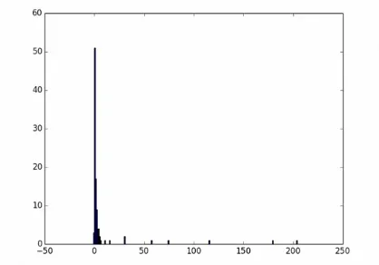
-1 3 0 51 1 17 2 9 3 4 4 4 5 2 6 1 10 1 15 1 30 2 57 1 74 1 115 1 179 1 203 1
Plot the Data
When people (or reindeer) work with data, their end goal is to uncover some answer or pattern. They most often employ Hadoop to turn big data into small data, then use traditional analytics techniques to turn small data into answers and insights. One such technique is to plot the information. If a picture is worth 1,000 words, then even a basic data plot is worth reams of statistical analysis.
That’s because the human eye often gets a rough idea of a pattern faster than people can write code to divine the proper mathematical result. A few lines of Python can create a histogram to present to our reindeer pals, to give a gestalt sense of UFO reporting delays.
To create a histogram chart, we’ll run a Python script on our docker gateway:
#!/usr/bin/python
# Example histogram: UFO reporting delay by day import numpy as np
To view the chart, we need to get the image back on your local machine, and then open it:
# Enter password 'chimpy'
scp -i insecure_key.pem -P 9022 chimpy@$DOCKER_IP:UFO_Reporting_Delays.png . open UFO_Reporting_Delays.png
Reindeer Conclusion
Hadoop Versus Traditional Databases
We’ve covered the basic operation of Hadoop MapReduce jobs on a Hadoop cluster, but it is worth taking a moment to reflect on how operating Hadoop differs from operating a traditional relational database. Hadoop is not a database.
Fundamentally, the storage engine at the heart of a traditional relational database does two things: it holds all the records, and it maintains a set of indexes for lookups and other operations (the crane arm in Santa’s legacy system). To retrieve a record, it must consult the appropriate index to find the
location of the record, then load it from the disk. This is very fast for record-by-record retrieval, but becomes cripplingly inefficient for general high-throughput access. If the records are stored by
location and arrival time (as the mailbags were on the Big Tree), then there is no “locality of access” for records retrieved by, say, type of toy — records for Lego will be spread all across the disk. With traditional drives, the disk’s read head has to physically swing back and forth in a frenzy across the drive platter, and though the newer flash drives have smaller retrieval latency, it’s still far too high for bulk operations.
What’s more, traditional database applications lend themselves very well to low-latency operations (such as rendering a web page showing the toys you requested), but very poorly to high-throughput operations (such as requesting every single doll order in sequence). Unless you invest specific expertise and effort, you have little ability to organize requests for efficient retrieval. You either suffer a variety of nonlocality-and-congestion-based inefficiencies, or wind up with an application that caters to the database more than to its users. You can to a certain extent use the laws of
economics to bend the laws of physics (as the commercial success of Oracle and Netezza shows), but the finiteness of time, space, and memory presents an insoluble scaling problem for traditional
databases.
The MapReduce Haiku
The bargain that MapReduce proposes is that you agree to only write programs fitting this haiku:
data flutters by
elephants make sturdy piles context yields insight
More prosaically, we might explain MapReduce in three phases.
Phase Description Explanation
Map Process and label Turn each input record into any number of labeled records
Group-sort Sorted context groups Hadoop groups those records uniquely under each label, in a sorted order (you’ll see this alsocalled the shuffle/sort phase)
Reduce Synthesize (process context
groups) For each group, process its records in order; emit anything you want
The trick lies in the group-sort (or shuffle/sort) phase: assigning the same label to two records in the map phase ensures that they will become local in the reduce phase.
The records in phase 1 (map) are out of context. The mappers see each record exactly once, but with no promises as to order, and no promises as to which mapper sees which record. We’ve moved the compute to the data, allowing each process to work quietly on the data in its workspace. Over at C&E, Inc., letters and translation passages aren’t preorganized and they don’t have to be; JT and Nanette care about keeping all the chimps working steadily and keeping the hallways clear of interoffice document requests.
Once the map attempt finishes, each partition (the collection of records destined for a common
reducer, with a common label, or key) is dispatched to the corresponding machine, and the mapper is free to start a new task. If you notice, the only time data moves from one machine to another is when the intermediate piles of data get shipped. Instead of an exhausted crane arm, we now have a
Map Phase, in Light Detail
Digging a little deeper into the mechanics of it all, a mapper receives one record at a time. By default, Hadoop works on text files, and a record is one line of text. However, there is a caveat: Hadoop actually supports other file formats and other types of storage beside files. But for the most part, the examples in this book will focus on processing files on disk in a readable text format. The whole point of the mapper is to “label” the record so that the shuffle/sort phase can track records with the same label.
Group-Sort Phase, in Light Detail
In the group-sort (or shuffle/sort) phase, Hadoop transfers all the map output records in a partition to the corresponding reducer. That reducer merges the records it receives from all mappers, so that each group contains all records for its label regardless of what machine it came from. What’s nice about the shuffle/sort phase is that you don’t have to do anything for it. Hadoop takes care of moving the data around for you. What’s less nice about the shuffle/sort phase is that it is typically the
Reduce Phase, in Light Detail
Whereas the mapper sees single records in isolation, a reducer receives one key (the label) and all
records that match that key. In other words, a reducer operates on a group of related records. Just as with the mapper, as long as it keeps eating records and doesn’t fail, the reducer can do anything with those records it pleases and emit anything it wants. It can emit nothing, it can contact a remote
database, it can emit nothing until the very end and then emit one or a zillion records. The output can be text, it can be video files, it can be angry letters to the president. They don’t have to be labeled, and they don’t have to make sense. Having said all that, usually what a reducer emits are nice well-formed records resulting from sensible transformations of its input, like the count of records, the
largest or smallest value from a field, or full records paired with other records. And though there’s no explicit notion of a label attached to a reducer output record, it’s pretty common that within the
record’s fields are values that future mappers will use to form labels.
Wrapping Up
You’ve just seen how records move through a MapReduce workflow, both in theory and in practice. This can be challenging material to grasp, so don’t feel bad if you don’t get all of it right away. While we did our best to simplify a complex phenomenon, we hope we’ve still communicated the essentials. We encourage you to reread this chapter until you get it straight. You may also try revisiting this
chapter after you’ve read a bit further in the book. Once you’ve performed a few Pig GROUP BYs, this
material may feel more natural.
You should now have an intuitive sense of the mechanics behind MapReduce Remember to come back to this chapter as you read the rest of the book. This will aide you in acquiring a deep
understanding of the operations that make up the strategies and tactics of the analytic toolkit. By the end of the book, you’ll be converting Pig syntax into MapReduce jobs in your head! You’ll be able to reason about the cost of different operations and optimize your Pig scripts accordingly.
Chapter 3. A Quick Look into Baseball
In this chapter, we will introduce the dataset we use throughout the book: baseball performance statistics. We will explain the various metrics used in baseball (and in this book), such that if you aren’t a baseball fan you can still follow along.
Nate Silver calls baseball the “perfect dataset.” There are not many human-centered systems for which this comprehensive degree of detail is available, and no richer set of tables for truly demonstrating the full range of analytic patterns.
The Data
Our baseball statistics come in tables at multiple levels of detail.
Putting people first as we like to do, the people table lists each player’s name and personal stats
(height and weight, birth year, etc.). It has a primary key, the player_id, formed from the first five
letters of the player’s last name, first two letters of their first name, and a two-digit disambiguation slug. There are also primary tables for ballparks (parks, which lists information on every stadium
that has ever hosted a game) and for teams (teams, which lists every Major League team back to the
birth of the game).
The core statistics table is bat_seasons, which gives each player’s batting stats by season (to
simplify things, we only look at offensive performance). The player_id and year_id fields form a
primary key, and the team_id foreign key represents the team that played the most games in a season.
The park_teams table lists, for each team, all “home” parks in which a player played by season,
along with the number of games and range of dates. We put “home” in quotes because technically it only signifies the team that bats last (a significant advantage), though teams nearly always play those home games at a single stadium in front of their fans. However, there are exceptions, as you’ll see in
Chapter 4. The park_id, team_id, and year_id fields form its primary key, so if a team did in fact
have multiple home ballparks, there will be multiple rows in the table.
There are some demonstrations where we need data with some real heft — not so much that you can’t run it on a single-node cluster, but enough that parallelizing the computation becomes important. In those cases, we’ll go to the games table (100+ MB), which holds the final box score summary of
every baseball game played, or to the full madness of the events table (1+ GB), which records every
play for nearly every game back to the 1940s and before. These tables have nearly 100 columns each in their original form. Not to carry the joke quite so far, we’ve pared them back to only a few dozen columns each, with only a handful seeing actual use.
Acronyms and Terminology
We use the following acronyms (and, coincidentally, field names) in our baseball dataset:
G Games
PA Plate appearances (the number of completed chances to contribute offensively; for historical reasons, some stats use a restricted
subset of plate appearances called AB, which stands for at bats, but should generally prefer PA to AB, and can pretend they
represent the same concept)
H Hits — the value for this can be h1B (a single), h2B (a double), h3B (a triple), or HR (a home run) BB Walks (pitcher presented too many unsuitable pitches)
HBP Hit by pitch (like a walk but more painful)
OBP On-base percentage (indicates effectiveness at becoming a potential run)
SLG Slugging percentage (indicates effectiveness at converting potential runs into runs) OPS On-base-plus-slugging (a reasonable estimate of overall offensive contribution)
For those uninterested in baseball or who consider sporting events to be the dull province of jocks: when we say that the “on-base percentage” is a simple matter of finding (H + BB + HBP) / AB, just
The Rules and Goals
Major League Baseball teams play a game nearly every single day from the start of April to the end of September (currently, 162 per season). The team on offense sends its players to bat in order, with the goal of having its players reach base and advance the full way around the diamond. Each time a
player makes it all the way to home, his team scores a run, and at the end of the game, the team with the most runs wins. We count these events as games (G), plate appearances on offense (PA), and runs
(R).
The best way to reach base is by hitting the ball back to the fielders and reaching base safely before they can retrieve the ball and chase you down — this is called a hit (H). You can also reach base on a
walk (BB) if the pitcher presents too many unsuitable pitches, or from a hit by pitch (HBP), which is
like a walk but more painful. You advance on the basepaths when your teammates hit the ball or reach base; the reason a hit is valuable is that you can advance as many bases as you can run in time. Most hits are singles (h1B) — batter safely reaches first base. Even better is for the batter to get a double
(h2B); a triple (h3B), which is rare and requires very fast running; or a home run (HR), usually by
clobbering the ball out of the park.
Your goal as a batter is twofold: you want to become a potential run and you want to help convert players on base into runs. If the batter does not reach base, it counts as an out, and after three outs, all the players on base lose their chance to score and the other team comes to bat. (This threshold
Performance Metrics
These baseball statistics are all “counting stats,” and generally, the more games, the more hits and runs and so forth. For estimating performance and comparing players, it’s better to use “rate stats” normalized against plate appearances.
On-base percentage (OBP) indicates how well the player meets offensive goal #1: get on base, thus
becoming a potential run and not consuming a precious out. It is given as the fraction of plate
appearances that are successful: ((H + BB + HBP) / PA).1 An OBP over 0.400 is very good (better
than 95% of significant seasons).
Slugging percentage (SLG) indicates how well the player meets offensive goal #2: advance the
runners on base, thus converting potential runs into points toward victory. It is given by the total bases gained in hitting (one for a single, two for a double, etc.) divided by the number of at bats: ((H + h2B + 2*h3B + 3*HR) / AB). An SLG over 0.500 is very good.
On-base-plus-slugging (OPS) combines on-base and slugging percentages to give a simple and useful
estimate of overall offensive contribution. It’s found by simply adding the figures: (OBP + SLG).
Anything above 0.900 is very good.
Just as a professional mechanic has an assortment of specialized and powerful tools, modern baseball analysis uses statistics significantly more nuanced than these. But when it comes time to hang a
picture, they use the same hammer as the rest of us. You might think that using the OBP, SLG, and OPS
Wrapping Up
In this chapter, we have introduced our dataset so that you can understand our examples without prior knowledge of baseball. You now have enough information about baseball and its metrics to work through the examples in this book. Whether you’re a baseball fan or not, this dataset should work well for teaching analytic patterns. If you are a baseball fan, feel free to filter the examples to tell stories about your favorite team.
In Part II, we’ll use baseball examples to teach analytic patterns — those operations that enable most kinds of analysis. First, though, we’re going to learn about Apache Pig, which will dramatically streamline our use of MapReduce.
1 Although known as percentages, OBP and SLG are always given as fractions to three decimal places. For OBP, we’re also using a slightly modified formula to reduce the number of stats to learn. It gives
Chapter 4. Introduction to Pig
In this chapter, we introduce the tools to teach analytic patterns in the chapters that comprise Part II of the book. To start, we’ll set you up with chains of MapReduce jobs in the form of Pig scripts, and then we’ll explain Pig’s data model and tour the different datatypes. We’ll also cover basic
operations like LOAD and STORE. Next, we’ll learn about UFOs and when people most often report
them, and we’ll dive into Wikipedia usage data and compare different projects. We’ll also briefly introduce the different kind of analytic operations in Pig that we’ll be covering in the rest of the book. Finally, we’ll introduce you to two libraries of user-defined functions (UDFs): the Apache DataFu project and the Piggybank.