Accounting: Focusing on the Elephants, Ignoring the
Mice
CRISTIAN ESTAN and GEORGE VARGHESE University of California, San Diego
Accurate network traffic measurement is required for accounting, bandwidth provisioning and detecting DoS attacks. These applications see the traffic as a collection of flows they need to measure. As link speeds and the number of flows increase, keeping a counter for each flow is too expensive (using SRAM) or slow (using DRAM). The current state-of-the-art methods (Cisco’s sampled NetFlow) which count periodically sampled packets are slow, inaccurate and resource-intensive. Previous work showed that at different granularities a small number of “heavy hitters” accounts for a large share of traffic. Our paper introduces a paradigm shift by concentrating the measurement process on large flows only — those above some threshold such as 0.1% of the link capacity.
We propose two novel and scalable algorithms for identifying the large flows: sample and hold
andmultistage filters, which take a constant number of memory references per packet and use a small amount of memory. IfMis the available memory, we show analytically that the errors of our new algorithms are proportional to 1/M; by contrast, the error of an algorithm based on classical sampling is proportional to 1/√M, thus providing much less accuracy for the same amount of memory. We also describe further optimizations such asearly removaland conservative update
that further improve the accuracy of our algorithms, as measured on real traffic traces, by an order of magnitude. Our schemes allow a new form of accounting calledthreshold accountingin which only flows above a threshold are charged by usage while the rest are charged a fixed fee. Threshold accounting generalizes usage-based and duration based pricing.
Categories and Subject Descriptors: C.2.3 [Computer-Communication Networks]: Network Operations—traffic measurement, identifying large flows
General Terms: Algorithms,Measurement
Additional Key Words and Phrases: Network traffic measurement, usage based accounting, scal-ability, on-line algorithms, identifying large flows
1. INTRODUCTION
If we’re keeping per-flow state, we have a scaling problem, and we’ll be tracking millions of ants to track a few elephants. — Van Jacobson, End-to-end Research meeting, June 2000.
Measuring and monitoring network traffic is required to manage today’s com-plex Internet backbones [Feldmann et al. 2000; Duffield and Grossglauser 2000]. Such measurement information is essential for short-term monitoring (e.g., detect-ing hot spots and denial-of-service attacks [Mahajan et al. 2001]), longer term traffic engineering (e.g., rerouting traffic[Shaikh et al. 1999] and upgrading selected links[Feldmann et al. 2000]), and accounting (e.g., to support usage based
ing[Duffield et al. 2001]).
The standard approach advocated by the Real-Time Flow Measurement (RTFM) [Brownlee et al. 1999] Working Group of the IETF is to instrument routers to add flow meters at either all or selected input links. Today’s routers offer tools such as NetFlow [NetFlow ] that give flow level information about traffic.
The main problem with the flow measurement approach is its lack ofscalability. Measurements on MCI traces as early as 1997 [Thomson et al. 1997] showed over 250,000 concurrent flows. More recent measurements in [Fang and Peterson 1999] using a variety of traces show the number of flows between end host pairs in a one hour period to be as high as 1.7 million (Fix-West) and 0.8 million (MCI). Even with aggregation, the number of flows in 1 hour in the Fix-West used by [Fang and Peterson 1999] was as large as 0.5 million.
It can be feasible for flow measurement devices to keep up with the increases in the number of flows (with or without aggregation) only if they use the cheapest memories: DRAMs. Updating per-packet counters in DRAM is already impossible with today’s line speeds; further, the gap between DRAM speeds (improving 7-9% per year) and link speeds (improving 100% per year) is only increasing. Cisco NetFlow [NetFlow ], which keeps its flow counters in DRAM, solves this problem by sampling: only sampled packets result in updates. But Sampled NetFlow has problems of its own (as we show later) since sampling affects measurement accuracy. Despite the large number of flows, a common observation found in many mea-surement studies (e.g., [Feldmann et al. 2000; Fang and Peterson 1999]) is that a small percentage of flows accounts for a large percentage of the traffic. [Fang and Peterson 1999] shows that 9% of the flows between AS pairs account for 90% of the byte traffic between all AS pairs.
For many applications, knowledge of these large flows is probably sufficient. [Fang and Peterson 1999; Pan et al. 2001] suggest achieving scalable differentiated services by providing selective treatment only to a small number of large flows. [Feldmann et al. 2000] underlines the importance of knowledge of “heavy hitters” for decisions about network upgrades and peering. [Duffield et al. 2001] proposes a usage sensi-tive billing scheme that relies on exact knowledge of the traffic of large flows but only samples of the traffic of small flows.
1.1 Problem definition
A flow is generically defined by an optionalpattern(which defines which packets we will focus on) and anidentifier(values for a set of specified header fields). We can also generalize by allowing the identifier to be afunctionof the header field values (e.g., using prefixes instead of addresses based on a mapping using route tables). Flow definitions vary with applications: for example for a traffic matrix one could use a wildcard pattern and identifiers defined by distinct source and destination network numbers. On the other hand, for identifying TCP denial of service attacks one could use a pattern that focuses on TCP packets and use the destination IP address as a flow identifier. Note that we do not require the algorithms to support simultaneously all these ways of aggregating packets into flows. The algorithms know a priori which flow definition to use and they do not need to ensure that a posteriori analyses based on different flow definitions are possible (as they are based on NetFlow data).
Large flows are defined as those that send more than a given threshold (say 0.1% of the link capacity) during a given measurement interval (1 second, 1 minute or even 1 hour). The technical report version of this paper [Estan and Varghese 2002] gives alternative definitions and algorithms based on defining large flows via leaky bucket descriptors.
An ideal algorithm reports, at the end of the measurement interval, the flow IDs and sizes of all flows that exceeded the threshold. A less ideal algorithm can fail in three ways: it can omit some large flows, it can wrongly add some small flows to the report, and can give an inaccurate estimate of the traffic of some large flows. We call the large flows that evade detectionfalse negatives, and the small flows that are wrongly includedfalse positives.
The minimum amount of memory required by an ideal algorithm is the inverse of the threshold; for example, there can be at most 1000 flows that use more than 0.1% of the link. We will measure the performance of an algorithm by four metrics: first, its memory compared to that of an ideal algorithm; second, the algorithm’s probability of false negatives; third, the algorithm’s probability of false positives; and fourth, the expected error in traffic estimates.
1.2 Motivation
Our algorithms for identifying large flows can potentially be used to solve many problems. Since different applications define flows by different header fields, we need a separate instance of our algorithms for each of them. Applications we envisage include:
—Scalable Threshold Accounting: The two poles of pricing for network traffic
importantly, for reasonably small values ofz (say 1%) threshold accounting may offer a compromise between that is scalable and yet offers almost the same utility as usage based pricing. [Altman and Chu 2001] offers experimental evidence based on the INDEX experiment that such threshold pricing could be attractive to both users and ISPs. 1
—Real-time Traffic Monitoring: Many ISPs monitor backbones for hot-spots
in order to identify large traffic aggregates that can be rerouted (using MPLS tunnels or routes through optical switches) to reduce congestion. Also, ISPs may consider sudden increases in the traffic sent to certain destinations (the victims) to indicate an ongoing attack. [Mahajan et al. 2001] proposes a mechanism that reacts as soon as attacks are detected, but does not give a mechanism to detect ongoing attacks. For both traffic monitoring and attack detection, it may suffice to focus on large flows.
—Scalable Queue Management: At a smaller time scale, scheduling
mecha-nisms seeking to approximate max-min fairness need to detect and penalize flows sending above their fair rate. Keeping per flow state only for these flows [Feng et al. 2001; Pan et al. 2001] can improve fairness with small memory. We do not address this application further, except to note that our techniques may be useful for such problems. For example, [Pan et al. 2001] uses classical sampling techniques to estimate the sending rates of large flows. Given that our algorithms have better accuracy than classical sampling, it may be possible to provide in-creased fairness for the same amount of memory by applying our algorithms.
The rest of the paper is organized as follows. We describe related work in Section 2, describe our main ideas in Section 3, and provide a theoretical analysis in Section 4. We theoretically compare our algorithms with NetFlow in Section 5. After showing how to dimension our algorithms in Section 6, we describe experi-mental evaluation on traces in Section 7. We end with implementation issues in Section 8 and conclusions in Section 9.
2. RELATED WORK
The primary tool used for flow level measurement by IP backbone operators is Cisco NetFlow [NetFlow ]. NetFlow keeps per flow counters in a large, slow DRAM. Ba-sic NetFlow has two problems: i) Processing Overhead: updating the DRAM slows down the forwarding rate; ii) Collection Overhead: the amount of data generated by NetFlow can overwhelm the collection server or its network connec-tion. For example [Feldmann et al. 2000] reports loss rates of up to 90% using basic NetFlow.
The processing overhead can be alleviated using sampling: per-flow counters are incrementedonlyfor sampled packets2. Classical random sampling introduces
considerable inaccuracy in the estimate; this is not a problem for measurements over long periods (errors average out) and if applications do not need exact data.
1Besides [Altman and Chu 2001], a brief reference to a similar idea can be found in [Shenker et al.
1996]. However, neither paper proposes a fast mechanism to implement the idea.
2NetFlow preforms 1 in N periodic sampling, but to simplify the analysis we assume in this paper
However, we will show that sampling does not work well for applications that require true lower bounds on customer traffic (e.g., it may be infeasible to charge customers based on estimates that are larger than actual usage) and for applications that require accurate data at small time scales (e.g., billing systems that charge higher during congested periods).
The data collection overhead can be alleviated by having the router aggregate flows (e.g., by source and destination AS numbers) as directed by a manager. How-ever, [Fang and Peterson 1999] shows that even the number of aggregated flows is very large. For example, collecting packet headers for Code Red traffic on a class A network [Moore 2001] produced 0.5 Gbytes per hour of compressed NetFlow data and aggregation reduced this data only by a factor of 4. Techniques described in [Duffield et al. 2001] can be used to reduce the collection overhead at the cost of further errors. However, it can considerablysimplifyrouter processing to only keep track of heavy-hitters (as in our paper) if that is what the application needs.
Many papers address the problem of mapping the traffic of large IP networks. [Feldmann et al. 2000] deals with correlating measurements taken at various points to find spatial traffic distributions; the techniques in our paper can be used to complement their methods. [Duffield and Grossglauser 2000] describes a mechanism for identifying packet trajectories in the backbone, that is not focused towards estimating the traffic between various networks. [Shaikh et al. 1999] proposes that edge routers identify large long lived flows and route them along less loaded paths to achieve stable load balancing. Our algorithms might allow the detection of these candidates for re-routing in higher speed routers too.
fil-ters we call conservative upsate. In [Karp et al. 2003] Karp et al. give an algorithm that is guaranteed to identify all elements that repeat frequently in a single pass. They use a second pass over the data to count exactly the number of occurrences of the frequent elements because the first pass does not guarantee accurate results. Building on our work, Narayanasamy et al. use [Narayanasamy et al. 2003] multi-stage filters with conservative update to determine execution profiles in hardware and obtain promising results.
3. OUR SOLUTION
Because our algorithms use an amount of memory that is a constant factor larger than the (relatively small) number of large flows, our algorithms can be implemented using on-chip or off-chip SRAM to store flow state. We assume that at each packet arrival we can afford to look up a flow ID in the SRAM, update the counter(s) in the entry or allocate a new entry if there is no entry associated with the current packet.
The biggest problem is to identify the large flows. Two approaches suggest them-selves. First, when a packet arrives with a flow ID not in the flow memory, we could make place for the new flow by evicting the flow with the smallest measured traffic (i.e., smallest counter). While this works well on traces, it is possible to provide counter examples where a large flow is not measured because it keeps being expelled from the flow memory before its counter becomes large enough. This can happen even when using an LRU replacement policy as in [Smitha et al. 2001].
A second approach is to use classical random sampling. Random sampling (simi-lar to sampled NetFlow except using a smaller amount of SRAM) provably identifies large flows. However, as the well known result from Table I shows, random sampling introduces a very high relative error in the measurement estimate that is propor-tional to 1/√M, whereM is the amount of SRAM used by the device. Thus one needs very high amounts of memory to reduce the inaccuracy to acceptable levels. The two most important contributions of this paper are two new algorithms for identifying large flows: Sample and Hold (Section 3.1) and Multistage Filters
(Section 3.2). Their performance is very similar, the main advantage of sample and hold being implementation simplicity, and the main advantage of multistage filters being higher accuracy. In contrast to random sampling, the relative errors of our two new algorithms scale with 1/M, where M is the amount of SRAM. This allows our algorithms to provide much more accurate estimates than random sampling using the same amount of memory. However, unlike sampled NetFlow, our algorithms access the memory for each packet, so they must use memories fast enough to keep up with line speeds. In Section 3.3 we present improvements that further increase the accuracy of these algorithms on traces (Section 7). We start by describing the main ideas behind these schemes.
3.1 Sample and hold
Base Idea: The simplest way to identify large flows is through sampling but with
F3 2 F1 3
F1 F1 F2 F3 F2 F4 F1 F3 F1 Entry updated
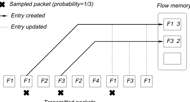
Sampled packet (probability=1/3)
Entry created
Transmitted packets
Flow memory
Fig. 1. The leftmost packet with flow labelF1 arrives first at the router. After an entry is created for a flow (solid line) the counter is updated for all its packets (dotted lines)
belonging to the flow as shown in Figure 1. The counting samples of Gibbons and Matias [Gibbons and Matias 1998] use the same core idea.
Thus once a flow is sampled, a corresponding counter is held in a hash table in flow memory till the end of the measurement interval. While this clearly requires processing (looking up the flow entry and updating a counter) for every packet (unlike Sampled NetFlow), we will show that the reduced memory requirements allow the flow memory to be in SRAM instead of DRAM. This in turn allows the per-packet processing to scale with line speeds.
Letpbe the probability with which we sample a byte. Thus the sampling prob-ability for a packet of sizes is ps = 1−(1−p)s ≈1−e−sp. This can be looked
up in a precomputed table or approximated byps=p∗s(for example for packets
of up to 1500 bytes and p ≤ 10−5 this approximation introduces errors smaller
than 0.76% inps). Choosing a high enough value forpguarantees that flows above
the threshold are very likely to be detected. Increasing p unduly can cause too many false positives (small flows filling up the flow memory). The advantage of this scheme is that it is easy to implement and yet gives accurate measurements with very high probability.
Preliminary Analysis: The following example illustrates the method and
anal-ysis. Suppose we wish to measure the traffic sent by flows that take over 1% of the link capacity in a measurement interval. There are at most 100 such flows. Instead of making our flow memory have just 100 locations, we will allow oversampling by a factor of 100 and keep 10,000 locations. We wish to sample each byte with probabilitypsuch that the average number of samples is 10,000. Thus ifC bytes can be transmitted in the measurement interval,p= 10,000/C.
For the error analysis, consider a flow F that takes 1% of the traffic. ThusF
All packets
Every xth Update entry or create a new one
Large flow packet
Large reports to
management station
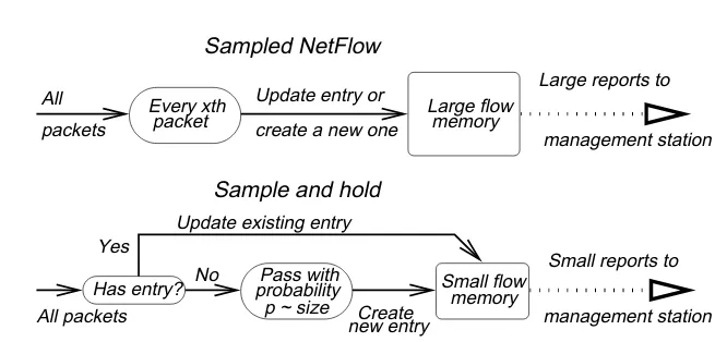
Sampled NetFlow
Sample and hold
memory
Yes
No
Update existing entry
Create
Small flow p ~ size
Pass with probability
management station Small reports to
new entry
memory All packets
Has entry?
Fig. 2. Sampled NetFlow counts only sampled packets, sample and hold counts all after entry created
end of the measurement interval (false negative) is (1−10000/C)C/100which is very
close to e−100. Notice that the factor of 100 in the exponent is the oversampling
factor. Better still, the probability that flowF is in the flow memory after sending 5% of its traffic is, similarly, 1−e−5 which is greater than 99% probability. Thus
with 99% probability the reported traffic for flowF will be at most 5% below the actual amount sent byF.
The analysis can be generalized to arbitrary threshold values; the memory needs to scale inversely with the threshold percentage and directly with the oversampling factor. Notice also that the analysis assumes that there is always space to place a sample flow not already in the memory. Setting p = 10,000/C ensures only that theaverage number of flows sampled3 is no more than 10,000. However, the
distribution of the number of samples is binomial with a small standard deviation (square root of the mean). Thus, adding a few standard deviations to the memory estimate (e.g., a total memory size of 10,300) makes it extremely unlikely that the flow memory will ever overflow4.
Compared to Sampled NetFlow our idea has three significant differences. Most importantly, we sample only to decide whether to add a flow to the memory; from that point on, we update the flow memory with every byte the flow sends as shown in Figure 2. As Section 5 shows this will make our results much more accurate. Second, our sampling technique avoids packet size biases unlike NetFlow which samples everyxpackets. Third, our technique reduces the extra resource overhead (router processing, router memory, network bandwidth) for sending large reports
3Our analyses from Section 4.1 and from [Estan and Varghese 2002] also give tight upper bounds
on the number of entries used that hold with high probability.
4If the flow memory overflows, we can not create new entries until entries are freed at the beginning
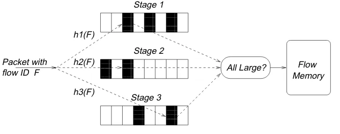
Packet with
Fig. 3. In a parallel multistage filter, a packet with a flow IDF is hashed using hash function
h1 into a Stage 1 table,h2 into a Stage 2 table, etc. Each table entry contains a counter that is incremented by the packet size. Ifallthe hashed counters are above the threshold (shown bolded),
F is passed to the flow memory for individual observation.
with many records to a management station.
3.2 Multistage filters
Base Idea: The basic multistage filter is shown in Figure 3. The building blocks
are hash stages that operate in parallel. First, consider how the filter operates with only one stage. A stage is a table of counters which is indexed by a hash function computed on a packet flow ID; all counters in the table are initialized to 0 at the start of a measurement interval. When a packet comes in, a hash on its flow ID is computed and the size of the packet is added to the corresponding counter. Since all packets belonging to the same flow hash to the same counter, if a flowF sends more than threshold T, F’s counter will exceed the threshold. If we add to the flow memory all packets that hash to counters ofT or more, we are guaranteed to identify all the large flows (no false negatives). The multi-stage algorithm of Fang et al [Fang et al. 1998] is similar to our multistage filters and the accounting bins of stochastic fair blue [Feng et al. 2001] use a similar data structure to compute drop probabilities for active queue management.
Unfortunately, since the number of counters we can afford is significantly smaller than the number of flows, many flows will map to the same counter. This can cause false positives in two ways: first, small flows can map to counters that hold large flows and get added to flow memory; second, several small flows can hash to the same counter and add up to a number larger than the threshold.
simple analysis.
Preliminary Analysis: Assume a 100 Mbytes/s link5, with 100,000 flows and
we want to identify the flows above 1% of the link during a one second measurement interval. Assume each stage has 1,000 buckets and a threshold of 1 Mbyte. Let’s see what the probability is for a flow sending 100 Kbytes to pass the filter. For this flow to pass one stage, the other flows need to add up to 1 Mbyte - 100 Kbytes = 900 Kbytes. There are at most 99,900/900=111 such buckets out of the 1,000 at each stage. Therefore, the probability of passing one stage is at most 11.1%. With 4 independent stages, the probability that a certain flow no larger than 100 Kbytes passes all 4 stages is the product of the individual stage probabilities which is at most 1.52∗10−4.
Based on this analysis, we can dimension the flow memory so that it is large enough to accommodate all flows that pass the filter. The expected number of flows below 100 Kbytes passing the filter is at most 100,000∗15.2∗10−4 < 16.
There can be at most 999 flows above 100 Kbytes, so the number of entries we expect to accommodate all flows is at most 1,015. Section 4 has a rigorous theorem that proves a stronger bound (for this example 122 entries) that holds for any distribution of flow sizes. Note the potential scalability of the scheme. If the number of flows increases to 1 million, we simply add a fifth hash stage to get the same effect. Thus to handle 100,000 flows requires roughly 4000 counters and a flow memory of approximately 100 memory locations, while to handle 1 million flows requires roughly 5000 counters and the same size of flow memory. This is logarithmic scaling.
The number of memory accesses per packet for a multistage filter is one read and one write per stage. If the number of stages is small, this is feasible even at high speeds by doing parallel memory accesses to each stage in a chip implementation.6
Multistage filters also need to compute the hash functions. These can be computed efficiently in hardware. For software implementations this adds to the per packet processing and can replace memory accesses as the main bottleneck. However, we already need to compute a hash function to locate the per flow entries in the flow memory, thus one can argue that we do not introduce a new problem, just make an existing one worse. While multistage filters are more complex than sample-and-hold, they have two important advantages. They reduce the probability of false negatives to 0 and decrease the probability of false positives, thereby reducing the size of the required flow memory.
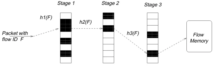
3.2.1 The serial multistage filter. We briefly present a variant of the multistage filter called a serial multistage filter (Figure 4). Instead of using multiple stages in parallel, we can place them serially after each other, each stage seeing only the packets that passed the previous stage.
Let d be the number of stages (the depth of the serial filter). We set a stage thresholdofT /dfor all the stages. Thus for a flow that sendsT bytes, by the time the last packet is sent, the counters the flow hashes to at alldstages reachT /d, so the packet will pass to the flow memory. As with parallel filters, we have no false
5To simplify computation, in our examples we assume that 1Mbyte=1,000,000 bytes and
1Kbyte=1,000 bytes.
Packet with
Fig. 4. In a serial multistage filter, a packet with a flow IDF is hashed using hash functionh1 into a Stage 1 table. If the counter is below the stage thresholdT /d, it is incremented. If the counter reaches the stage threshold the packet is hashed using functionh2 to a Stage 2 counter, etc. If the packet passes all stages, an entry is created forF in the flow memory.
negatives. As with parallel filters, small flows can pass the filter only if they keep hashing to counters made large by other flows.
The analytical evaluation of serial filters is more complicated than for parallel filters. On one hand the early stages shield later stages from much of the traffic, and this contributes to stronger filtering. On the other hand the threshold used by stages is smaller (by a factor ofd) and this contributes to weaker filtering. Since, as shown in Section 7, parallel filters perform better than serial filters on traces of actual traffic, the main focus in this paper will be on parallel filters.
3.3 Improvements to the basic algorithms
The improvements to our algorithms presented in this section further increase the accuracy of the measurements and reduce the memory requirements. Some of the improvements apply to both algorithms, some apply only to one of them.
3.3.1 Basic optimizations. There are a number of basic optimizations that ex-ploit the fact that large flows often last for more than one measurement interval.
Preserving entries: Erasing the flow memory after each interval implies that
the bytes of a large flow sent before the flow is allocated an entry are not counted. By preserving entries of large flows across measurement intervals and only reini-tializing stage counters, all long lived large flows are measured nearly exactly. To distinguish between a large flow that was identified late and a small flow that was identified by error, a conservative solution is to preserve the entries of not only the flows for which we count at leastT bytes in the current interval, but also all the flows that were added in the current interval (since they may be large flows that entered late).
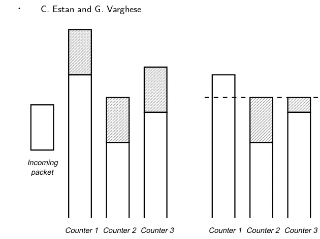
Early removal: Sample and hold has a larger rate of false positives than
0000
Counter 1 Counter 2 Counter 3 Counter 1 Counter 2 Counter 3
Fig. 5. Conservative update: without conservative update (left) all counters are increased by the size of the incoming packet, with conservative update (right) no counter is increased to more than the size of the smallest counter plus the size of the packet
Shielding: Consider large, long lived flows that go through the filter each
mea-surement interval. Each meamea-surement interval, the counters they hash to exceed the threshold. With shielding, traffic belonging to flows that have an entry in flow memory no longer passes through the filter (the counters in the filter are not in-cremented for packets with an entry), thereby reducing false positives. If we shield the filter from a large flow, many of the counters it hashes to will not reach the threshold after the first interval. This reduces the probability that a random small flow will pass the filter by hashing to counters that are large because of other flows.
3.3.2 Conservative update of counters. We now describe an important optimiza-tion for multistage filters that improves performance by an order of magnitude.
Conservative update reduces the number of false positives of multistage filters by three subtle changes to the rules for updating counters. In essence, we endeavour to increment counters as little as possible (thereby reducing false positives by pre-venting small flows from passing the filter) while still avoiding false negatives (i.e., we need to ensure that all flows that reach the threshold still pass the filter.)
The first change (Figure 5) applies only to parallel filters and only for packets that don’t pass the filter. As usual, an arriving flowF is hashed to a counter at each stage. We update the smallest of the counters normally (by adding the size of the packet). However, the other counters are set to the maximum of their old value and the new value of the smallest counter. Since the amount of traffic sent by the current flow is at most the new value of the smallest counter, this change
The second change is very simple and applies to both parallel and serial filters. When a packet passes the filter and it obtains an entry in the flow memory, no counters should be updated. This will leave the counters below the threshold. Other flows with smaller packets that hash to these counters will get less “help” in passing the filter.
The third change applies only to serial filters. It regards the way counters are updated when the threshold is exceeded in any stage but the last one. Let’s say the value of the counter a packet hashes to at stageiisT /d−xand the size of the packet is s > x >0. Normally one would increment the counter at stage i toT /d
and adds−xto the counter from stagei+ 1. What we can do instead with the counter at stagei+ 1 is update its value to the maximum ofs−xand its old value (assumings−x < T /d). Since the counter at stageiwas belowT /d, we know that no prior packets belonging to the same flow as the current one passed this stage and contributed to the value of the counter at stagei+ 1. We could not apply this change if the thresholdT was allowed to change during a measurement interval.
4. ANALYTICAL EVALUATION OF OUR ALGORITHMS
In this section we analytically evaluate our algorithms. We only present the main results. The proofs, supporting lemmas and some of the less important results (e.g. high probability bounds corresponding to our bounds on the average number of flows passing a multistage filter) are in [Estan and Varghese 2002]. We focus on two important questions:
—How good are the results? We use two distinct measures of the quality of the results: how many of the large flows are identified, and how accurately is their traffic estimated?
—What are the resources required by the algorithm? The key resource measure is the size of flow memory needed. A second resource measure is the number of memory references required.
In Section 4.1 we analyze our sample and hold algorithm, and in Section 4.2 we analyze multistage filters. We first analyze the basic algorithms and then examine the effect of some of the improvements presented in Section 3.3. In the next section (Section 5) we use the results of this section to analytically compare our algorithms with sampled NetFlow.
Example: We will use the following running example to give numeric instances. Assume a 100 Mbyte/s link with 100,000 flows. We want to measure all flows whose traffic is more than 1% (1 Mbyte) of link capacity in a one second measurement interval.
4.1 Sample and hold
We first define some notation we use in this section.
—pthe probability for sampling a byte; —sthe size of a flow (in bytes);
—T the threshold for large flows;
—C the capacity of the link – the number of bytes that can be sent during the
—O the oversampling factor defined byp=O·1/T; —cthe number of bytes actually counted for a flow.
4.1.1 The quality of results for sample and hold. The first measure of the quality of the results is the probability that a flow at the threshold is not identified. As presented in Section 3.1 the probability that a flow of size T is not identified is (1−p)T ≈e−O. An oversampling factor of 20 results in a probability of missing
flows at the threshold of 2∗10−9.
Example: For our example,pmust be 1 in 50,000 bytes for an oversampling of 20. With an average packet size of 500 bytes this is roughly 1 in 100 packets.
The second measure of the quality of the results is the difference between the size of a flow sand our estimate. The number of bytes that go by before the first one gets sampled has a geometric probability distribution7: it isxwith a probability8
(1−p)xp.
ThereforeE[s−c] = 1/pandSD[s−c] =√1−p/p. The best estimate forsis
c+ 1/pand its standard deviation is√1−p/p. If we choose to usecas an estimate forsthen the error will be larger, but we never overestimate the size of the flow9.
In this case, the deviation from the actual value of s is pE[(s−c)2] =√2−p/p.
Based on this value we can also compute the relative error of a flow of sizeT which isT√2−p/p=√2−p/O.
Example: For our example, with an oversampling factor O of 20, the relative error (computed as the standard deviation of the estimate divided by the actual value) for a flow at the threshold is 7%.
4.1.2 The memory requirements for sample and hold. The size of the flow mem-ory is determined by the number of flows identified. The actual number of sampled packets is an upper bound on the number of entries needed in the flow memory because new entries are created only for sampled packets. Assuming that the link is constantly busy, by the linearity of expectation, the expected number of sampled bytes isp·C=O·C/T.
Example: Using an oversampling of 20 requires 2,000 entries on average. The number of sampled bytes can exceed this value. Since the number of sampled bytes has a binomial distribution, we can use the normal curve to bound with high probability the number of bytes sampled during the measurement interval. Therefore with probability 99% the actual number will be at most 2.33 standard deviations above the expected value; similarly, with probability 99.9% it will be at most 3.08 standard deviations above the expected value. The standard deviation of the number of sampled bytes isp
Cp(1−p).
Example: For an oversampling of 20 and an overflow probability of 0.1% we need at most 2,147 entries.
7We ignore for simplicity that the bytes before the first sampled byte that are in the same packet
with it are also counted. Therefore the actual algorithm will be more accurate than this model.
8Since we focus on large flows, we ignore for simplicity the correction factor we need to apply to
account for the case when the flow goes undetected (i.e. xis actually bound by the size of the flows, but we ignore this).
9Gibbons and Matias [Gibbons and Matias 1998] have a more elaborate analysis and use a different
This result can be further tightened if we make assumptions about the distribu-tion of flow sizes and thus account for very large flows having many of their packets sampled. Let’s assume that the flows have a Zipf (Pareto) distribution with param-eter 1 defined asP rs > x=constant∗x−1. If we havenflows that use the whole
bandwidthC, the total traffic of the largestj flows is at leastClnln(2(jn+1)+1)[Estan and Varghese 2002]. For any value of j between 0 and n we obtain an upper bound on the number of entries expected to be used in the flow memory by assuming that the largestj flows always have an entry by having at least one of their pack-ets sampled and each packet sampled from the rest of the traffic creates an entry:
j+Cp(1−ln(j+ 1)/ln(2n+ 1). By differentiating we obtain the value ofj that provides the tightest bound: j=Cp/ln(2n+ 1)−1.
Example: Using an oversampling of 20 requires at most 1,328 entries on average.
4.1.3 The effect of preserving entries. We preserve entries across measurement intervals to improve accuracy. The probability of missing a large flow decreases because we cannot miss it if we keep its entry from the prior interval. Accuracy increases because we know the exact size of the flows whose entries we keep. To quantify these improvements we need to know the ratio of long lived flows among the large ones.
The cost of this improvement in accuracy is an increase in the size of the flow memory. We need enough memory to hold the samples from both measurement intervals10. Therefore the expected number of entries is bounded by 2O·C/T.
To bound with high probability the number of entries we use the normal curve and the standard deviation of the number of sampled packets during the 2 intervals which isp
2Cp(1−p).
Example: For an oversampling of 20 and acceptable probability of overflow equal to 0.1%, the flow memory has to have at most 4,207 entries to preserve entries.
4.1.4 The effect of early removal. The effect of early removal on the proportion of false negatives depends on whether or not the entries removed early are reported. Since we believe it is more realistic that implementations will not report these entries, we will use this assumption in our analysis. LetR < T be the early removal threshold. A flow at the threshold is not reported unless one of its first T −R
bytes is sampled. Therefore the probability of missing the flow is approximately
e−O(T−R)/T. If we use an early removal threshold ofR= 0.2∗T, this increases the
probability of missing a large flow from 2∗10−9to 1.1∗10−7with an oversampling
of 20.
Early removal reduces the size of the memory required by limiting the number of entries that are preserved from the previous measurement interval. Since there can be at mostC/R flows sendingR bytes, the number of entries that we keep is at mostC/Rwhich can be smaller thanOC/T, the bound on the expected number of sampled packets. The expected number of entries we need isC/R+OC/T.
To bound with high probability the number of entries we use the normal curve. IfR≥T /O the standard deviation is given only by the randomness of the packets
10We actually also keep the older entries that are above the threshold. Since we are performing
sampled in one interval and ispCp(1−p).
Example: An oversampling of 20 andR = 0.2T with overflow probability 0.1% requires 2,647 memory entries.
4.2 Multistage filters
In this section, we analyze parallel multistage filters. We first define some new notation:
—bthe number of buckets in a stage;
—dthe depth of the filter (the number of stages); —nthe number of active flows;
—kthe stage strength is the ratio of the threshold and the average size of a counter.
k= T bC , whereC denotes the channel capacity as before. Intuitively, this is the factor we inflate each stage memory beyond the minimum ofC/T .
Example: To illustrate our results numerically, we will assume that we solve the measurement example described in Section 4 with a 4 stage filter, with 1000 buckets at each stage. The stage strengthkis 10 because each stage memory has 10 times more buckets than the maximum number of flows (i.e., 100) that can cross the specified threshold of 1%.
4.2.1 The quality of results for multistage filters. As discussed in Section 3.2, multistage filters have no false negatives. The error of the traffic estimates for large flows is bounded by the thresholdT since no flow can sendT bytes without being entered into the flow memory. The stronger the filter, the less likely it is that the flow will be entered into the flow memory much before it reachesT. We first state an upper bound for the probability of a small flow passing the filter described in Section 3.2.
Lemma 1. Assuming the hash functions used by different stages are independent, the probability of a flow of sizes < T(1−1/k)passing a parallel multistage filter is
at mostps≤
1 kTT−s
d .
The proof of this bound formalizes the preliminary analysis of multistage filters from Section 3.2. Note that the boundmakes no assumption about the distribution of flow sizes, and thus applies for all flow distributions. We only assume that the hash functions are random and independent. The bound is tight in the sense that it is almost exact for a distribution that has⌊(C−s)/(T−s)⌋flows of size (T−s) that send all their packets before the flow of sizes. However, for realistic traffic mixes (e.g., if flow sizes follow a Zipf distribution), this is a very conservative bound.
Based on this lemma we obtain a lower bound for the expected error for a large flow.
Theorem 2. The expected number of bytes of a large flow of size sundetected by a multistage filter is bound from below by
E[s−c]≥T
1− d
k(d−1)
−ymax (1)
This bound suggests that we can significantly improve the accuracy of the esti-mates by adding a correction factor to the bytes actually counted. The down side to adding a correction factor is that we can overestimate some flow sizes; this may be a problem for accounting applications. The ymax factor from the result comes
from the fact that when the packet that makes the counters exceed the threshold arrives,c is initialized to its size which can be as much asymax.
4.2.2 The memory requirements for multistage filters. We can dimension the flow memory based on bounds on the number of flows that pass the filter. Based on Lemma 1 we can compute a bound on the total number of flows expected to pass the filter (the full derivation of this theorem is in Appendix A).
Theorem 3. The expected number of flows passing a parallel multistage filter is bound by
E[npass]≤max b k−1, n
n kn−b
d!
+n
n kn−b
d
(2)
Example: Theorem 3 gives a bound of 121.2 flows. Using 3 stages would have resulted in a bound of 200.6 and using 5 would give 112.1. Note that when the first term dominates the max, there is not much gain in adding more stages.
We can also bound the number of flows passing the filter with high probability.
Example: The probability that more than 185 flows pass the filter is at most 0.1%. Thus by increasing the flow memory from the expected size of 122 to 185 we can make overflow of the flow memory extremely improbable.
As with sample and hold, making assumptions about the distribution of flow sizes can lead to a smaller bound on the number of flows expected to enter the flow memory[Estan and Varghese 2002].
Theorem 4. If the flows sizes have a Zipf distribution with parameter 1, the expected number of flows passing a parallel multistage filter is bound by
E[npass]≤i0+ n
kd + db kd+1 +
db ln(n+ 1)d−2
k2k ln(n+ 1)− b i0−0.5
d−1 (3)
wherei0=⌈max(1.5 +k ln(bn+1),ln(2n+1)(b k−1))⌉.
Example: Theorem 4 gives a bound of 21.7 on the number of flows expected to pass the filter.
4.2.3 The effect of preserving entries and shielding. Preserving entries affects the accuracy of the results the same way as for sample and hold: long lived large flows have their traffic counted exactly after their first interval above the threshold. As with sample and hold, preserving entries basically doubles all the bounds for memory usage.
Shielding has a strong effect on filter performance, since it reduces the traffic presented to the filter. Reducing the trafficαtimes increases the stage strength to
Measure Sample Multistage Sampling and hold filters
Relative error for a flow of sizezC √2 M z
1+10r log10(n)
M z
1
√
M z
Memory accesses per packet 1 1 +log10(n) 1x= M C
Table I. Comparison of the core algorithms: sample and hold provides most accurate results while pure sampling has very few memory accesses
5. COMPARING MEASUREMENT METHODS
In this section we analytically compare the performance of three traffic measurement algorithms: our two new algorithms (sample and hold and multistage filters) and Sampled NetFlow. First, in Section 5.1, we compare the algorithms at the core of traffic measurement devices. For the core comparison, we assume that each of the algorithms is given thesameamount of high speed memory and we compare their accuracy and number of memory accesses. This allows a fundamental analytical comparison of the effectiveness of each algorithm in identifying heavy-hitters.
However, in practice, it may be unfair to compare Sampled NetFlow with our algorithms using the same amount of memory. This is because Sampled NetFlow can afford to use a large amount of DRAM (because it does not process every packet) while our algorithms cannot (because they process every packet and hence need to store per flow entries in SRAM). Thus we perform a second comparison in Section 5.2 of complete traffic measurement devices. In this second comparison, we allow Sampled NetFlow to use more memory than our algorithms. The comparisons are based on the algorithm analysis in Section 4 and an analysis of NetFlow taken from [Estan and Varghese 2002].
5.1 Comparison of the core algorithms
In this section we compare sample and hold, multistage filters and ordinary sam-pling (used by NetFlow) under the assumption that they are all constrained to usingM memory entries. More precisely, the expected number of memory entries used is at most M irrespective of the distribution of flow sizes. We focus on the accuracy of the measurement of a flow (defined as the standard deviation of an estimate over the actual size of the flow) whose traffic iszC (for flows of 1% of the link capacity we would usez= 0.01).
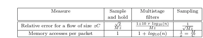
The bound on the expected number of entries is the same for sample and hold and for sampling and is pC. By making this equal to M we can solve forp. By substituting in the formulae we have for the accuracy of the estimates and after eliminating some terms that become insignificant (as pdecreases and as the link capacity goes up) we obtain the results shown in Table I.
For multistage filters, we use a simplified version of the result from Theorem 3:
E[npass]≤b/k+n/kd. We increase the number of stages used by the multistage
filter logarithmically as the number of flows increases so that only a single small flow is expected to pass the filter11and the strength of the stages is 10. At this point we
11Configuring the filter such that a small number of small flows pass would have resulted in
Measure Sample and hold Multistage filters Sampled NetFlow Exact measurements /longlived% longlived% 0
Relative error 1.41/O / 1/u 0.0088/
√
zt
Memory bound 2O/z 2/z+ 1/z log10(n) min(n,486000 t)
Memory accesses 1 1 +log10(n) 1/x
Table II. Comparison of traffic measurement devices
estimate the memory usage to beM =b/k+ 1 +rbd=C/T+ 1 +r10log10(n)C/T
where r < 1 depends on the implementation and reflects the relative cost of a counter and an entry in the flow memory. From here we obtainT which will be an upper bound on the error of our estimate of flows of sizezC. From here, the result from Table I is immediate.
The termM zthat appears in all formulae in the first row of the table is exactly equal to the oversampling we defined in the case of sample and hold. It expresses how many times we are willing to allocate over the theoretical minimum memory to obtain better accuracy. We can see that the error of our algorithms decreases inversely proportional to this term while the error of sampling is proportional to the inverse of its square root.
The second line of Table I gives the number of memory locations accessed per packet by each algorithm. Since sample and hold performs a packet lookup for every packet12, its per packet processing is 1. Multistage filters add to the one
flow memory lookup an extra access to one counter per stage and the number of stages increases as the logarithm of the number of flows. Finally, for ordinary sampling one inx=C/Mpackets get sampled so the average per packet processing is 1/x=M/C.
Table I provides a fundamental comparison of our new algorithms with ordinary sampling as used in Sampled NetFlow. The first line shows that the relative error of our algorithms scales with 1/M which is much better than the 1/√M scaling of ordinary sampling. However, the second line shows that this improvement comes at the cost of requiring at least one memory access per packet for our algorithms. While this allows us to implement the new algorithms using SRAM, the smaller number of memory accesses (≪ 1) per packet allows Sampled NetFlow to use DRAM. This is true as long as x is larger than the ratio of a DRAM memory access to an SRAM memory access. However, even a DRAM implementation of Sampled NetFlow has some problems which we turn to in our second comparison.
5.2 Comparing Measurement Devices
Table I implies that increasing DRAM memory sizeM to infinity can reduce the relative error of Sampled NetFlow to zero. But this assumes that by increasing memory one can increase the sampling rate so that xbecomes arbitrarily close to 1. If x= 1, there would be no error since every packet is logged. But xmust at
12We equate a lookup in the flow memory to a single memory access. This is true if we use
least be as large as the ratio of DRAM speed (currently around 60 ns) to SRAM speed (currently around 5 ns); thus Sampled NetFlow will always have a minimum error corresponding to this value ofxeven when given unlimited DRAM.
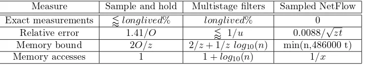
With this insight, we now compare the performance of our algorithms and Net-Flow in Table II without limiting NetNet-Flow memory. Thus Table II takes into ac-count the underlying technologies (i.e., the potential use of DRAM over SRAM) and one optimization (i.e., preserving entries) for both of our algorithms.
We consider the task of estimating the size of all the flows above a fractionz of the link capacity over a measurement interval oft seconds. In order to make the comparison possible we change somewhat the way NetFlow operates: we assume that it reports the traffic data for each flow after each measurement interval, like our algorithms do. The four characteristics of the traffic measurement algorithms presented in the table are: the percentage of large flows known to be measured exactly, the relative error of the estimate of a large flow, the upper bound on the memory size and the number of memory accesses per packet.
Note that the table does not contain the actual memory used but a bound. For example the number of entries used by NetFlow is bounded by the number of active flows and the number of DRAM memory lookups that it can perform during a measurement interval (which doesn’t change as the link capacity grows)13. Our
measurements in Section 7 show that for all three algorithms the actual memory usage is much smaller than the bounds, especially for multistage filters. Memory is measured in entries, not bytes. We assume that a flow memory entry is equivalent to 10 of the counters used by the filter (i.e. r = 1/10) because the flow ID is typically much larger than the counter. Note that the number of memory accesses required per packet does not necessarily translate to the time spent on the packet because memory accesses can be pipelined or performed in parallel.
We make simplifying assumptions about technology evolution. As link speeds increase, so must the electronics. Therefore we assume that SRAM speeds keep pace with link capacities. We also assume that the speed of DRAM does not improve significantly ([Patterson and Hennessy 1998] states that DRAM speeds improve only at 9% per year while clock rates improve at 40% per year).
We assume the following configurations for the three algorithms. Our algorithms preserve entries. For multistage filters we introduce a new parameter expressing how many times larger a flow of interest is than the threshold of the filteru=zC/T. Since the speed gap between the DRAM used by sampled NetFlow and the link speeds increases as link speeds increase, NetFlow has to decrease its sampling rate proportionally with the increase in capacity14to provide the smallest possible error.
For the NetFlow error calculations we also assume that the size of the packets of large flows is 1500 bytes.
Besides the differences that stem from the core algorithms (Table I), we see new differences in Table II. The first big difference (Row 1 of Table II) is that unlike
13The limit on the number of packets NetFlow can process we used for Table II is based on Cisco
documentation that states that sampling should turned on for speeds larger than OC-3 (155.52 Mbits/second). Thus we assumed that this is the ,maximum speed at which NetFlow can handle minimum sized (40 byte) packets.
14If the capacity of the link isx times OC-3, then one inxpackets gets sampled. We assume
NetFlow, our algorithms provide exact measures for long-lived large flowsby pre-serving entries. More precisely, by prepre-serving entries our algorithms will exactly measure traffic for all (or almost all in the case of sample and hold) of the large flows that were large in the previous interval. Given that our measurements show that most large flows are long lived (depending on the flow definition, the average percentage of the large flows that were large in the previous measurement interval is between 56% and 81%), this is a big advantage.
Of course, one could get the same advantage by using an SRAM flow memory that preserves large flows across measurement intervals in Sampled NetFlow as well. However, that would require the router to root through its DRAM flow memory before the end of the interval to find the large flows, a large processing load. One can also argue that if one can afford an SRAM flow memory, it is quite easy to do sample and hold.
The second big difference (Row 2 of Table II) is that we can make our algorithms arbitrarily accurate at the cost of increases in the amount of memory used15 while
sampled NetFlow can do so only by increasing the measurement intervalt. The third row of Table II compares the memory used by the algorithms. The extra factor of 2 for sample and hold and multistage filters arises from preserving entries. Note that the number of entries used by Sampled NetFlow is bounded by both the numbernof active flows and the number of memory accesses that can be made intseconds. Finally, the fourth row of Table II is identical to the second row of Table I.
Table II demonstrates that our algorithms have two advantages over NetFlow: i)they provide exact values for long-lived large flows (row 1) andii)they provide much better accuracy even for small measurement intervals (row 2). Besides these advantages, our algorithms also have three more advantages not shown in Table II. These are iii) provable lower bounds on traffic, iv) reduced resource consump-tion for collecconsump-tion, and v) faster detection of new large flows. We now examine advantagesiii)throughv)in more detail.
iii) Provable Lower Bounds: A possible disadvantage of Sampled NetFlow is
that the NetFlow estimate is not an actual lower bound on the flow size. Thus a customer may be charged for more than the customer sends. While one can make the probability of overcharging arbitrarily low (using large measurement intervals or other methods from [Duffield et al. 2001]), there may be philosophical objections to overcharging. Our algorithms do not have this problem.
iv) Reduced Resource Consumption: Clearly, while Sampled NetFlow can
increase DRAM to improve accuracy, the router has more entries at the end of the measurement interval. These records have to be processed, potentially aggregated, and transmitted over the network to the management station. If the router extracts the heavy hitters from the log, then router processing is large; if not, the bandwidth consumed and processing at the management station is large. By using fewer entries, our algorithms avoid these resource (e.g., memory, transmission bandwidth, and router CPU cycles) bottlenecks, but as detailed in Table II sample and hold and multistage filters incur more upfront work by processing each packet.
15Of course, technology and cost impose limitations on the amount of available SRAM but the
ADAPTTHRESHOLD
usage=entriesused/f lowmemsize
if (usage > target)
threshold=threshold∗(usage/target)adjustup else
if (threshold did not increase for 3 intervals)
threshold=threshold∗(usage/target)adjustdown endif
endif
Fig. 6. Dynamic threshold adaptation to achieve target memory usage
6. DIMENSIONING TRAFFIC MEASUREMENT DEVICES
We describe how to dimension our algorithms. For applications that face adversarial behavior (e.g., detecting DoS attacks), one should use the conservative bounds from Sections 4.1 and 4.2. Other applications such as accounting can obtain greater accuracy from more aggressive dimensioning as described below. The measurements from Section 7 show that the gains can be substantial. For example the number of false positives for a multistage filter can be four orders of magnitude below what the conservative analysis predicts. To avoid a priori knowledge of flow distributions, we adapt algorithm parameters to actual traffic. The main idea is tokeep decreasing the threshold below the conservative estimate until the flow memory is nearly full
(totally filling the memory can result in new large flows not being tracked). Dynamically adapting the threshold is an effective way to control memory usage. Sampled NetFlow uses a fixed sampling rate that is either so low that a small percentage of the memory is used all or most of the time, or so high that the memory is filled and NetFlow is forced to expire entries which might lead to inaccurate results exactly when they are most important: when the traffic surges.
Figure 6 presents our threshold adaptation algorithm. There are two important constants that adapt the threshold to the traffic: the “target usage” (variabletarget
in Figure 6) that tells it how full the memory can be without risking filling it up completely and the “adjustment ratio” (variables adjustup and adjustdown
in Figure 6) that the algorithm uses to decide how much to adjust the threshold to achieve a desired increase or decrease in flow memory usage. To give stability to the traffic measurement device, the entriesused variable does not contain the number of entries used over the last measurement interval, but an average of the last 3 intervals.
to a value of 3 foradjustup, 1 foradjustdownin the case of sample and hold and 0.5 for multistage filters.
6.1 Dimensioning the multistage filter
Even if we have the correct constants for the threshold adaptation algorithm, there are other configuration parameters for the multistage filter we need to set. Our aim in this section is not to derive the exact optimal values for the configuration parameters of the multistage filters. Due to the dynamic threshold adaptation, the device will work even if we use suboptimal values for the configuration parameters. Nevertheless we want to avoid using configuration parameters that would lead the dynamic adaptation to stabilize at a value of the threshold that is significantly higher than the one for the optimal configuration.
We assume that design constraints limit the total amount of memory we can use for the stage counters and the flow memory, but we have no restrictions on how to divide it between the filter and the flow memory. Since the number of per packet memory accesses might be limited, we assume that we might have a limit on the number of stages. We want to see how we should divide the available memory between the filter and the flow memory and how many stages to use. We base our configuration parameters on some knowledge of the traffic mix (the number of active flows and the percentage of large flows that are long lived).
We first introduce a simplified model of how the multistage filter works. Mea-surements confirm this model is closer to the actual behavior of the filters than the conservative analysis. Because of shielding the old large flows do not affect the filter. We assume that because of conservative update only the counters to which the new large flows hash reach the threshold. Letl be the number of large flows and ∆l be the number of new large flows. We approximate the probability of a small flow passing one stage by ∆l/b and of passing the whole filter by (∆l/b)d.
This gives us the number of false positives in each interval f p =n(∆l/b)d. The
number of memory locations used at the end of a measurement interval consists of the large flows and the false positives of the previous interval and the new large flows and the new false positives m =l+ ∆l+ 2∗f p. To be able to establish a tradeoff between using the available memory for the filter or the flow memory, we need to know the relative cost of a counter and a flow entry. Letrdenote the ratio between the size of a counter and the size of an entry. The amount of memory used by the filter is going to be equivalent to b∗d∗r entries. To determine the optimal number of counters per stage given a certain number of large flows, new large flows and stages, we take the derivative of the total memory with respect to
b. Equation 4 gives the optimal value for band Equation 5 gives the total amount of memory required with this choice ofb.
b= ∆ld+1 r
2n
r∆l (4)
mtotal=l+ ∆l+ (d+ 1)r∆ld +1
r
2n
r∆l (5)
(re-lated to the flow arrival rate) doesn’t depend on the threshold. Measurements confirm that this is a good approximation for wide ranges of the threshold. For the MAG trace, when we define the flows at the granularity of TCP connections ∆l/l
is around 44%, when defining flows based on destination IP 37% and when defining them as AS pairs 19%. LetM be the number of entries the available memory can hold. We solve Equation 5 with respect tol for all possible values ofd from 2 to the limit on the number of memory accesses we can afford per packet. We choose the depth of the filter that gives the largestland computebbased on that value.
7. MEASUREMENTS
In Section 4 and Section 5 we usedtheoreticalanalysis to understand the effective-ness of our algorithms. In this section, we turn toexperimental analysis to show that our algorithms behave much better on real traces than the (reasonably good) bounds provided by the earlier theoretical analysis and compare them with Sampled NetFlow.
We start by describing the traces we use and some of the configuration details common to all our experiments. In Section 7.1.1 we compare the measured per-formance of the sample and hold algorithm with the predictions of the analytical evaluation, and also evaluate how much the various improvements to the basic algo-rithm help. In Section 7.1.2 we evaluate the multistage filter and the improvements that apply to it. We conclude with Section 7.2 where we compare complete traffic measurement devices using our two algorithms with Cisco’s Sampled NetFlow.
We use 3 unidirectional traces of Internet traffic: a 4515 second “clear” one (MAG+) from CAIDA (captured in August 2001 on an OC-48 backbone link be-tween two ISPs) and two 90 second anonymized traces from the MOAT project of NLANR (captured in September 2001 at the access points to the Internet of two large universities on an OC-12 (IND) and an OC-3 (COS)). For some of the experiments use only the first 90 seconds of trace MAG+ as trace MAG.
In our experiments we use 3 different definitions for flows. The first definition is at the granularity of TCP connections: flows are defined by the 5-tuple of source and destination IP address and port and the protocol number. This definition is close to that of Cisco NetFlow. The second definition uses the destination IP address as a flow identifier. This is a definition one could use to identify at a router ongoing (distributed) denial of service attacks. The third definition uses the source and destination autonomous system as the flow identifier. This is close to what one would use to determine traffic patterns in the network. We cannot use this definition with the anonymized traces (IND and COS) because we cannot perform route lookups on them.
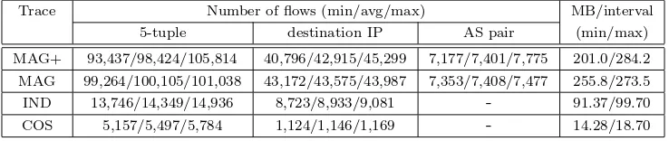
Table III describes the traces we used. The number of active flows is given for all applicable flow definitions. The reported values are the smallest, largest and average value over the measurement intervals of the respective traces. The number of megabytes per interval is also given as the smallest, average and largest value. Our traces use only between 13% and 27% of their respective link capacities.
Trace Number of flows (min/avg/max) MB/interval
5-tuple destination IP AS pair (min/max)
MAG+ 93,437/98,424/105,814 40,796/42,915/45,299 7,177/7,401/7,775 201.0/284.2 MAG 99,264/100,105/101,038 43,172/43,575/43,987 7,353/7,408/7,477 255.8/273.5
IND 13,746/14,349/14,936 8,723/8,933/9,081 - 91.37/99.70
COS 5,157/5,497/5,784 1,124/1,146/1,169 - 14.28/18.70
Table III. The traces used for our measurements
0 5 10 15 20 25 30
Percentage of flows 50
60 70 80 90 100
Percentage of traffic MAG 5-tuples MAG destination IP MAG AS pairs IND COS
Fig. 7. Cumulative distribution of flow sizes for various traces and flow definitions
packets (weighted by packet size) arrive within 5 seconds of the previous packet belonging to the same flow.
Since our algorithms are based on the assumption that a few heavy flows dominate the traffic mix, we find it useful to see to what extent this is true for our traces. Figure 7 presents the cumulative distributions of flow sizes for the traces MAG, IND and COS for flows defined by 5-tuples. For the trace MAG we also plot the distribution for the case where flows are defined based on destination IP address, and for the case where flows are defined based on the source and destination ASes. As we can see, the top 10% of the flows represent between 85.1% and 93.5% of the total traffic validating our original assumption that a few flows dominate.
7.1 Comparing Theory and Practice
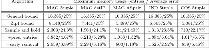
Algorithm Maximum memory usage (entries)/ Average error
MAG 5tuple MAG dstIP MAG ASpair IND 5tuple COS 5tuple
General bound 16,385/25% 16,385/25% 16,385/25% 16,385/25% 16,385/25% Zipf bound 8,148/25% 7,441/25% 5,489/25% 6,303/25% 5,081/25% Sample and hold 2,303/24.3% 1,964/24.1% 714/24.40% 1,313/23.8% 710/22.17%
+pres. entries 3,832/4.67% 3,213/3.28% 1,038/1.32% 1,894/3.04% 1,017/6.6% +early removal 2,659/3.89% 2,294/3.16% 803/1.18% 1,525/2.92% 859/5.46%
Table IV. Summary of sample and hold measurements for a threshold of 0.025% and an oversampling of 4
7.1.1 Summary of findings about sample and hold. Table IV summarizes our results for a single configuration: a threshold of 0.025% of the link with an over-sampling of 4. We ran 50 experiments (with different random hash functions) on each of the reported traces with the respective flow definitions. The table gives the maximum memory usage over the 900 measurement intervals and the ratio between average error for large flows and the threshold.
The first row presents thetheoretical bounds that hold without making any as-sumption about the distribution of flow sizes and the number of flows. These are not the bounds on the expected number of entries used (which would be 16,000 in this case), but high probability bounds.
The second row presentstheoreticalbounds assuming that we know the number of flows and know that their sizes have a Zipf distribution with a parameter of
α= 1. Note that the relative errors predicted by theory may appear large (25%) but these are computed for a very low threshold of 0.025% and only apply to flows exactly at the threshold.16
The third row shows the actual values we measured for the basic sample and hold algorithm. The actual memory usage is much below the bounds. The first reason is that the links are lightly loaded and the second reason (partially captured by the analysis that assumes a Zipf distribution of flows sizes) is that large flows have many of their packets sampled. The average error is very close to its expected value.
The fourth row presents the effects of preserving entries. While this increases memory usage (especially where large flows do not have a big share of the traffic) it significantly reduces the error for the estimates of the large flows, because there is no error for large flows identified in previous intervals. This improvement is most noticeable when we have many long lived flows.
The last row of the table reports the results when preserving entries as well as using an early removal threshold of 15% of the threshold (see Appendix B for why this is a good value). We compensated for the increase in the probability of false negatives early removal causes by increasing the oversampling to 4.7. The average error decreases slightly. The memory usage decreases, especially in the cases where
16We defined the relative error by dividing the average error by the size of the threshold. We
1 2 3 4 Depth of filter
0.001 0.01 0.1 1 10 100
Percentage of false positives (log scale)
General bound Zipf bound Serial filter Parallel filter Conservative update
Fig. 8. Filter performance for a stage strength of k=3
preserving entries caused it to increase most.
We performed measurements on many more configurations. The results are in general similar to the ones from Table IV, so we only emphasize some noteworthy differences. First, when the expected error approaches the size of a packet, we see significant decreases in the average error. Our analysis assumes that we sample at the byte level. In practice, if a certain packet gets sampled all its bytes are counted, including the ones before the byte that was sampled.
Second, preserving entries reduces the average error by 70% - 95% and increases memory usage by 40% - 70%. These figures do not vary much as we change the threshold or the oversampling. Third, an early removal threshold of 15% reduces the memory usage by 20% - 30%. The size of the improvement depends on the trace and flow definition and it increases slightly with the oversampling.
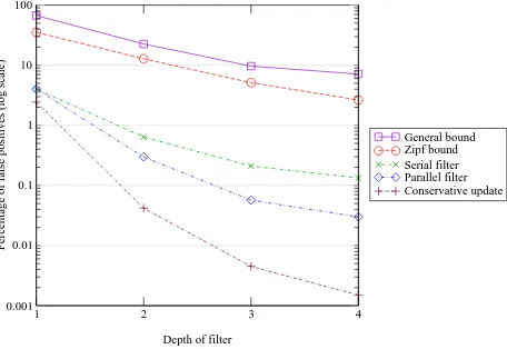
7.1.2 Summary of findings about multistage filters. Figure 8 summarizes our findings about configurations with a stage strength ofk= 3 for our most challenging trace: MAG with flows defined at the granularity of TCP connections. It represents the percentage of small flows (log scale) that passed the filter for depths from 1 to 4 stages. We used a threshold of a 4096th of the maximum traffic. The first (i.e., topmost and solid) line represents the bound of Theorem 3. The second line below represents the improvement in the theoretical bound when we assume a Zipf distribution of flow sizes. Unlike in the case of sample and hold we used the maximum traffic, not the link capacity for computing the theoretical bounds. This results in much tighter theoretical bounds.
![[Zuber Skerritt] New Directions in Action Research](data:image/gif;base64,R0lGODlhAQABAIAAAP///wAAACH5BAEAAAAALAAAAAABAAEAAAICRAEAOw==)