Geochemical and Geophysical Methodologies in Geothermal Exploration

Geochemical and Geophysical Methodologies in

Geothermal Exploration

Geophysical Methods in Geothermal Exploration

by

Adele Manzella

Italian National Research Council

CONTENTS

Contents 1

1. Introduction 2

2. Subsurface temperature and thermal gradient surveys 7

3. Gravity methods 11

4. Magnetic methods 11

5. Seismic methods 13

5.1 Active seismic methods 13

5.2 Passive seismic methods 17

6. Geophysical well logging 19

7. Electrical methods 20

7.1 Natural source methods (magnetotelluric and self-potential) 22

7.1.1 Magnetotelluric method 22

7.1.2 Self-potential method 31

7.2 Electromagnetic methods 32

7.3 Direct current methods 36

7.4 Modelling and Inversion 38

1. INTRODUCTION

Geophysical methods play a key role in geothermal exploration since many objectives of geothermal exploration can be achieved by these methods. The geophysical surveys are directed at obtaining indirectly, from the surface or from shallow depth, the physical parameters of the geothermal systems.

A geothermal system is made up of four main elements: a heat source, a reservoir, a fluid, which is the carrier that transfers the heat, and a recharge area. The heat source is generally a shallow magmatic body, usually cooling and often still partially molten. The volume of rocks from which heat can be extracted is called the geothermal reservoir, which contains hot fluids, a summary term describing hot water, vapour and gases. A geothermal reservoir is usually surrounded by colder rocks that are hydraulically connected with the reservoir. Hence water may move from colder rocks outside the reservoir (recharge) towards the reservoir, where hot fluids move under the influence of buoyancy forces towards a discharge area.

The first aspect of defining a geothermal system is the practical one of how much power can be produced. In most cases, the principal reason for developing geothermal energy is to produce electric power, although as an alternative the geothermal heat could be used in process applications or space heating. The typical geothermal system used for electric power generation must yield approximately 10 kg of steam to produce one unit (kWh) of electricity. Production of large quantities of electricity, at rates of hundreds of megawatts, requires the production of great volumes offluid. Thus, one aspect of a geothermal system is that it must contain great volumes of fluid at high temperatures or a reservoir that can be recharged with fluids that are heated by contact with the rock. A geothermal reservoir should lie at depths that can be reached by drilling. It is unreasonable to expect to find a hidden geothermal reservoir at depths of less than 1 km; at the present time it is not feasible to search for geothermal reservoirs that lie at depths of more than 3 or 4 km.

Experience has shown that each well drilled in a geothermal field must be capable of supporting 5 MW of electrical production; this corresponds to a steam production of 10 tonnes/h. To accomplish this, a well must penetrate permeable zones, usually fractures, that can support a high rate of flow. In many geothermal fields the wells are spaced so as to produce 25 – 30 MW km-2. At a few locations, where the reservoir consists of a highly fractured and shattered rock and there is little interference between wells, production rates may reach several hundred megawatts per square kilometre over small areas.

The geological setting in which a geothermal reservoir is to be found can vary widely. The largest geothermal fields currently under exploitation occur in rocks that range from limestone to shale, volcanic rock and granite. Volcanic rocks are probably the most common single rock type in which reservoirs occur. Rather than being identified with a specific lithology, geothermal reservoirs are more closely associated with heat flow systems. Many of the developed geothermal reservoirs around the world occur in convection systems in which hot water rises from deep within the earth and is trapped in reservoirs whose cap rock has been formed by silicification, or precipitation of other mineral elements. As far as geology is concerned, therefore, the important factors in identifying a geotherma1 reservoir are not rock units, but rather the existence of tectonic elements such as fracturing, and the presence of high heat flow.

Geothermal energy can also occur in areas where thick blankets of thermally insulating sediment cover basement rock that has a relatively normal heat flow. Geothermal systems based on the thermal blanket model are generally of lower grade than those of volcanic origin.

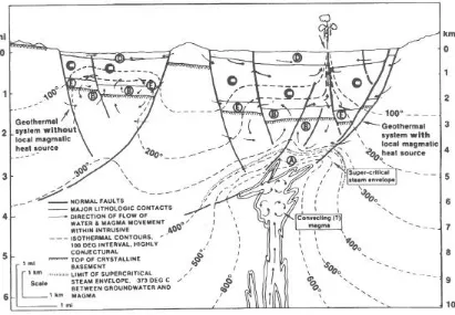
An important element in any model of a geothermal system in a vo1canic area is the source for the system: in other words, the existence of an intruded hot rock mass beneath the area where the shallower reservoirs are expected to occur. The source of a geothermal system could be either a pluton or a complex of dykes, depending upon the rock type injected (see Fig. 1).

Figure 1. Diagrammatic cross sections of hypothetical geothermal systems. The system on the left is not closely associated to an intrusion but results from higher than normal thermal gradients through a sequence of thermally resistant rocks. The system on the right has an intrusion as the heat source.

changes to have taken place in the physical, chemical and geological characteristics of the rock, all of which can be used in the exploration project.

Heat is not easily confined in small volumes of rock. Rather, heat diffuses readily, and a large volume of a rock around a geothermal system will have its properties altered. The rock volume in which anomalies in properties are to be expected will, therefore, generally be large. Exploration techniques need not offer a high level of resolution. Indeed, in geothermal exploration we prefer an approach that is capable of providing a high level of confidence that geothermal fluids will be recovered on drilling.

A geothermal assessment programme on a regional basis will begin with a review and coordination of the existing data. All heat flow data acquired previously will have to be re-evaluated, re-gridded, smoothed, averaged and plotted out in a variety of forms in an attempt to identify areas with higher than normal average heat flow. Similarly, the volumes of volcanic products with ages younger than 106 years should be tabulated in a similar way to provide a longer-range estimate of anomalous heat flow from the crust. Because fracturing is important, levels of seismicity should be analysed, averaged and presented in a uniform format. All information on thermal springs and warm springs should be quantified in some form and plotted in the same format. Comparison of these four sets of data, which relate directly to the characteristics of the basic geothermal model described above, will produce a pattern that will indicate whether the area possesses the conditions favourable for the occurrence of specific geothermal reservoirs. These areas should then be tested further by applying some or all of the many geophysical, geological and geochemical techniques designed to locate specific reservoirs from which fluids can be produced.

The next stage of exploration consists of techniques for detecting the presence of a geothermal system. A geothermal system generally causes inhomogeneities in the physical properties of the subsurface, which can be observed to varying degrees as anomalies measurable from the surface.

These physical parameters include temperature (thermal survey), electrical conductivity (electrical and electromagetic methods), elastic properties influencing the propagation velocity of elastic waves (seismic survey), density (gravity survey) and magnetic susceptibility (magnetic survey). Most of these methods can provide valuable information on the shape, size, and depth of the deep geological structures constituting a geothermal reservoir, and sometimes of the heat source. An increase of silica amount in volcanic rocks decreases the density. Thermal surveys can delimit the areas of enhanced thermal gradient, which is a basic requirement for high-enthalpy geothermal systems, and define temperature distribution. Information on the existence of geothermal fluids in the geological structures can be obtained with the electrical and electromagnetic prospectings, which are more sensitive than other surveys to the presence of these fluids, especially if salty, and to variations in temperature. Moreover resistivity are strongly affected by porosity and saturation. Resistivity decreases with increasing porosity and increasing saturation.

The same parameters measured indirectly from the surface can also be obtained from wells, by the method known as geophysical logging.

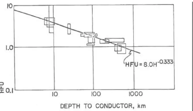
Fig. 2. Observed correlation between the depth to thermally excited conductive zone in the crust or mantle (based on magnetotelluric soundings) and heat flow.

The Curie point method has the potential for providing confirmation of the existence of a hot rock mass in the crust. When rocks are heated above temperatures of a few hundred degrees Centigrade, they lose their ferromagnetism. Under favourable circumstances, the depth to this demagnetisation level can be determined with reasonable accuracy.

Further confirmation can be obtained by p-wave delay and shear wave shadow studies. (When an anomalously hot mass of rock is present in the ground, the compressional (p) waves from earthquakes are delayed in transit, while the shear (s) waves are reduced in amplitude). To detect such an effect, an array of seismograph stations is set up in the vicinity of an anomaly. The seismograph stations are operated over a sufficiently long time to record a few tens of teleseisms. The wave speeds for various ray paths through the suspected anomalous zone are then computed; if the rock is partially molten, the p-wave velocities will be from 20 to 30 per cent lower than their normal values. An increase of silica amount in volcanic rocks decreases the p-wave velocity. Moreover seismic velocity is strongly affected by porosity and saturation. Wave velocity is reduced by increasing porosity but shows different behaviour for different saturation, with an inverse relationship when saturation is high (100/85%) and a direct relationship when saturation is low, being constant for saturation of 15-85%.

A group of prospect areas should be defined, with reference to regional data and reconnaisance surveys. These areas may range in size from a few hundred to a thousand km2. In rare cases, such as extensive thermal systems, they may be even larger. With the lack of resolution characteristic of the reconnaissance studies, it is unlikely that a prospect can be localised to an area of less than 100 km2. Detailed geophysical, geological and geochemical studies will be needed in order to identify drilling locations once a prospect area has been defined from reconnaissance.

geothermometer calculations carried out. Some prospect areas will probably show much more positive geochemical indicators than others. This could merely reflect the difference in the amount of leakage from subsurface reservoirs, but it does provide a basis for setting priorities for further testing; the geothermal reservoirs that show the most positive indications from geochemical thermometry should be the ones that are investigated first by other geophysical techniques.

The sequence in which geophysical methods are applied depends to a considerable extent on the specific characteristics of each prospect. It is not wise to define a particular sequence of geophysical surveys as being applicable to all potential reservoirs. In some cases, for example where we expect to find a subsurface convection system, various types of electrical survey could be highly effective in delineating the boundaries of the convecting system. Where large clay masses are present in the prospect area, on the other hand, electrical resistivity surveys can be deceptive. The particular type of electrical resistivity survey used at this stage is a matter of personal preference. Schlumberger sounding, dipole – dipole surveys, dipole mapping surveys and electromagnetic soundings can all be used to good effect. To some extent the choice of method here depends upon accessibility. The dipole–dipole traversing method and the Schlumberger sounding method are much more demanding in terms of access across the surface. The dipole mapping method and the electromagnetic sounding method can be applied in much more rugged terrain.

The objective when carrying out electrical surveys is to outline an area of anomalously low resistivity associated with a subsurface geothermal reservoir. When such an area has been identified, it is still necessary to confirm that the resistivity anomaly is the result of temperature and to locate areas within the anomaly where fracture permeability is likely to be high. Confirmation of subsurface temperatures is best done at this stage by drilling one or more heat flow boreholes. These heat flow holes need be only a few hundred metres deep if the area is one in which surface groundwater circulation is minimal. However, in volcanic areas where groundwater circulation occurs down to great depths, reliable heat flow data can be obtained only by drilling to one or two kilometres depth, in which case the heat flow hole becomes a reservoir test hole.

The number of heat flow holes that need to be drilled in a given prospect can vary widely; a single highly positive heat flow hole may be adequate in some cases while in others we may need several tens of heat flow holes to present convincing evidence for the presence of a geothermal reservoir at greater depth.

Once the probable existence of a geothermal reservoir has been established by a combination of resistivity studies and heat flow determinations, it is advisable to search for zones of fracture permeability in the reservoir before selecting a site for a test hole.

Microseismic surveys are a widely used tool for studying activity in fracture zones in a prospect area. Surveys may require many weeks of observation in a given area. The accuracy with which active faults can be located using microearthquakes is often not good enough for the control of drill holes, although in some cases it is adequate. A potentially valuable by-product of a microearthquake survey is the determination of Poisson’s ratio and related rock properties along various transmission paths through the potential geothermal system. Poisson’s ratio and attenuation of seismic waves can be strongly affected by fracturing. The identification of anomalous areas of Poisson’s ratio and p-wave attenuation can provide encouraging evidence for high permeability zones in the reservoir.

technique can be applied to detect faults through the disruption to the continuity of the bedding. The seismic reflection technique is extremely expensive, and a survey over a geothermal prospect may cost a significant fraction of the cost of a test well, but the results obtained with the seismic reflection method are usually much more conclusive than the results obtained with any other geophysical technique.

All of these geophysical surveys, targetted at defining the main characteristics of the geothermal reservoir, can also be supplemented with other types of geophysical surveys that assist us in understanding the regional geology and the local geological structure in a geothermal prospect. The self-potential survey is useful for our understanding of groundwater movement in an area. The gravity survey can be used to study the depth of fill in intermontaine valleys, and to locate intrusive masses of rock. Magnetic surveys can be used to identify the boundaries to flows in volcanic areas. Once all these detailed geophysical surveys have been carried out, a convincing set of data should be available before the decision is taken to locate a drill hole. There must be evidence for heat, there must be evidence for permeability, and the conditions for drilling must be established. Once we have achieved these objectives, we can tackle the problem of whether to drill a deep test well or not.

It is surprisingly difficult to record a true bottomhole temperature during the course of drilling a well. Mud is circulated through the well and removes much of the excess temperature as drilling progresses. In a closely controlled drilling programme, the temperature and volume of mud supplied to the well and recovered from the drilling operation should be monitored closely. Differences in the temperature between the mud going in and the mud coming back to the surface can be used to estimate bottomhole temperatures in a crude fashion. With the development of a mathematical model for the loss of heat from the rock to the drilling mud, it is conceivable that an even more precise temperature estimate will be attainable. The best temperature estimates during drilling are obtained by lowering maximum-reading thermometers to wellbottom whenever the bit has to be removed from the well for some reason. Several thermometers should be inserted at the same time in case one breaks or provides a false reading. They should be lowered to wellbottom on a heavy weight so as to be positioned as close as possible to the undisturbed rock at the bottom face of the borehole.

The following sections give a detailed review of the various geophysical techniques used in geothermal exploration, with particular emphasis on the requirements for data acquisition, handling, processing and interpretation.

2. SUBSURFACE TEMPERATURE AND THERMAL GRADIENT SURVEYS

the temperature gradients have either to be measured at a depth beyond which the contribution from surface temperature changes is insignificant, or in such a way that the surficial effects can be removed. For example, if temperatures are measured at the bottom of shallow holes over a period of one year, then the annual temperature can be averaged out. Alternatively, if measurements are made at depths beyond which the annual wave penetrated significantly, the normal heat flow from the interior of the earth will be detected in a matter of a few days. It is still a matter of debate as to which approach is more effective.

Our objective in the case of thermal gradient measurements in boreholes is twofold: first, to detect areas of unusually high temperature, and second, to determine quantitatively the component of heat flow along the direction of the borehole. Unusually high temperatures could indicate the presence of geothermal activity. More quantitative results are obtained when thermal gradients are converted to heat flow through the use of Fourier’s equation:

grad T = Φ/K

or

∆T/∆z = Φz/K

where ∆T/∆z is the vertical gradient in temperature, K is the thermal conductivity and Φz is

the thermal flux in the z direction. Thermal conductivity is measured in lab over rock samples, whereas temperature is measured in the well. The advantage of converting temperature gradients to heat flow values is that we eliminate the dependence on the thermal conductivity of the rock type. Thus, minor differences in temperature over a series of prospect holes can have added significance if we know that the differences are due not to a change in rock type, but to a change in the total amount of heat being supplied from beneath.

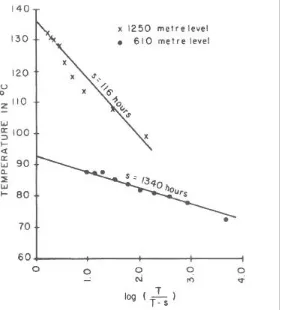
Determination of temperature in a test hole is not as easy as it might seem. In deep test holes, which must be drilled with a circulating fluid such as mud, a considerable disturbance of the normal temperature environment will take place during drilling. This is particularly true if the gradient is relatively high and the temperature change over the well interval is relatively large. As a rule of thumb, one must wait a period of time comparable to that involved in drilling the well before the well temperatures return to within 10 per cent of their undisturbed state. Drilling a well to several hundred metres depth may take a few days. In order to measure temperatures accurately for thermal gradient purposes we have to record downhole temperatures for periods that are several times longer than the duration of drilling. Fortunately there are a number of methods available for predicting stabilisation temperatures in a well. One such method consists of measuring temperatures at a given depth several times after completion of drilling. Temperatures are then plotted as a function of time on a linearising scale, defined as log T/(T – _{s), where T is the total time since the}

drill first opened the borehole at the depth where the temperature is being measured, and s

re-equilibration process. An example of the use of this method is shown in Fig. 3.

Fig. 3. Extrapolation of borehole temperatures to equilibrium temperature at two depths in a borehole drilled at the summit of Kilauea volcano (Hawaii). The parameter s is the duration of circulation in the well following first penetration by drill bit, and T is the total time elapsed from first penetration to measurement of temperature.

After extrapolation to equilibrium temperature, other corrections must be applied to temperature gradient to determine the heat flow. These are the paleoclimatic correction, the topographic correction and the correction due to changes of ground surface due to rapid sedimentation or erosion. Topographic correction takes into account the temperature variation due to valleys and mountains. Indeed, isotherms follow the topography, raising below mountains and lowering below valleys. In many methods the external temperature is considered constant or a certain temperature distribution at surface is considered. The reference plane is then the horizontal one at the measuring site and crossing topography. This correction takes into account the shape of topography and its changes in the time, as long as isotherms are in equilibrium. However, when these changes are rapid equilibrium is not reached and corrections due to sedimentation or erosion must be considered.

Paleoclimatic variations can be corrected using a schematic model where continuos climatic variations are taken into account and surface temperature is assumed constant in the last 10000 years.

The main difficulty in measuring heat flow in drill holes is that, in many geothermal fields, convection as well as conduction contributes significantly to total heat flow. Where convection is rapid, Fourier’s simple equation cannot be used to compute heat flow. Convection is not easily computed since hydrogeological conditions are not well known. Heat transfer by convection can be computed by theoretical models. On the contrary, the extension and importance of circulation is defined comparing the observed situation with the theoretical model based on the assumption of simple conduction.

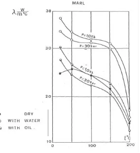
After all this corrections are applied to temperature, temperature gradient can be computed. To define the heat flow, however, thermal conductivity must be known. Another major problem in computing the heat flow is due to the variation of thermal conductivity, which can be measured many times and then averaged. Moreover conductivity decreases with temperature and increases with pressure. Variation due to pressure can be neglected since pressure changes very little at the depths involved in the investigation. Temperature variation can not be neglected and depends also on the saturation level (see Fig. 4).

Fig. 4. Thermal conductivity variation with temperature and pressure.

When thermal conductivity and temperature gradients are known, heat flow is mapped and anomalous areas are easily detected. Anomalies are linked to any heat source: however, those due to hot fluid circulation affect large areas. This way the most interesting areas can be defined and application of more expensive geophysical methods are limited.

3. GRAVITY SURVEYS

Gravity surveys are used during geothermal exploration to define lateral density variation related to deep magmatic body, which may represent the heat source. These anomalies can be created also by different degrees of differentiation of magma or varaition in depth of crust-mantle interface which creates also depth variation of isotherms.

Gravity monitoring surveys are mainly performed in geothermal areas to define the change in groundwater level and for subsidence monitoring. Fluid extraction from the ground which is not rapidly replaced causes an increase of pore pressure and hence of density. This effect may arrive at surface and produce a subsidence, whose rate depends on the recharge rate of fluid in the extraction area and the rocks interested by compaction.

Repeated gravity monitoring associated to weather monitoring may define the relationship between gravity and precipitation which produces the shallow ground water level change. When gravity is corrected by this effect, gravity changes show how much of the water mass discharged to the atmosphere is replaced by natural inflow. The underground hydrological monitoring done by gravity survey is an important indication of the fluid recharge in geothermal systems and the need of reinjection.

4. MAGNETIC SURVEYS

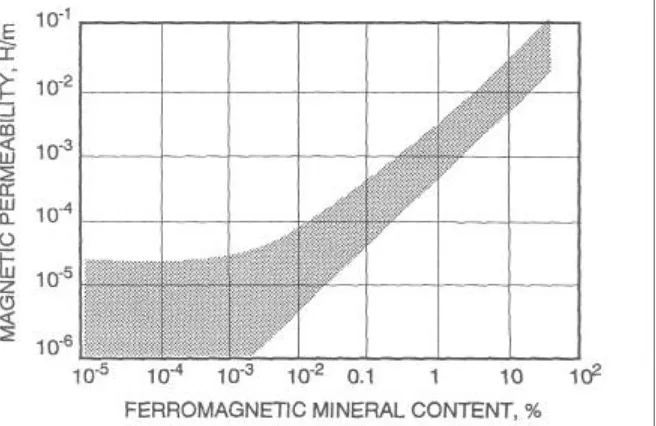
Surveys of the spatial changes in the strength of the magnetic field over the surface of the earth have been used as a method for geophysical exploration for many years. Magnetite is the most common ferromagnetic mineral and so, in most cases, the magnetic permeability is controlled by the presence of varying amounts of magnetite and related minerals in the rock ( Fig. 5). The magnetic method has come into use for identifying and locating masses of igneous rocks that have relatively high concentrations of magnetite. Strongly magnetic rocks include basalt and gabbro, while rocks such as granite, granodiorite and rhyolite have only moderately high magnetic susceptibilities.

The magnetic method is useful in mapping near-surface volcanic rocks that are often of interest in geothermal exploration, but the greatest potential for the method lies in its ability to detect the depth at which the Curie temperature is reached. Ferromagnetic materials exhibit a phenomenon characterised by a loss of nearly all magnetic susceptibility at a critical temperature called the Curie temperature. Various ferromagnetic minerals have differing Curie temperatures, but the Curie temperature of titano-magnetite, the most common magnetic minera1 in igneous rocks, is in the range of a few hundred to 570°C. The ability to determine the depth to the Curie point would be an ability to determine the depth to the Curie point isotherm as well.

bottom of the magnetised layer in the crust can be used to separate magnetic effects at the two depths and to determine the Curie point depth.

Fig. 5. Correlation between magnetic permeability and the content of ferromagnetic minerals in instrusive rocks.

The magnetic field of the earth is of a complex nature because of its dipolarity. The inducing magnetic field has a dip angle that varies from place to place over the surface of the earth, and this feature introduces a complexity into the patterns of anomalies that are recorded. This problem has long been recognised in the analysis of magnetic data, and a procedure has been developed to recompute the magnetic profile map for a vertical inducing field using the actual observed magnetic map. This first step in processing magnetic data is termed the conversion of the magnetic map ’to the pole’, or to the form it would have for a vertical inducing field.

5. SEISMIC METHODS

These methods can be divided into two main subclasses: passive seismic methods, which deal with the effects of natural earthquakes or those induced by fracturing related to geothermal fluid extraction and injection; and active seismic methods, which cover all seismic prospectings having an artificial wave source.

5. 1 PASSIVE SEISMIC METHODS

It has been observed by many researchers that geothermal systems occur mainly in areas characterised by a relatively high level of microseismic activity. However, in detail there does not appear to be a one-to-one relationship between the locations of microearthquakes and the presence of geothermal reservoirs. The identification of microearthquakes in a prospect area serves primarily as a means of investigating and characterising modern tectonic activity, which may be controlled by the same factors that control the emplacement of a geothermal system; in particularly favourable circumstances, studies of microseismic activity can serve as a guide when drilling into fractured rocks in a geothermal reservoir whose production levels are expected to be high.

In order for the location of microearthquakes to serve as an effective exploration tool, it is necessary that a relatively large number of events be recorded over a reasonable recording period in a survey area. The procedure normally used at present is to deploy a number of highly sensitive seismograph units in a prospect area. The number may range from 6 to 12 or more. The distance between any pair of seismographs should be no more than 5 – 10 km.

to be recorded at each seismometer. This assumption is not obviously valid, but programs to determine epicentres when there are lateral variations in wavespeed have not yet come into general use.

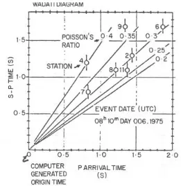
In locating an epicentre, the unknowns to be determined are the x, y, and z coordinates of the origin, the time at which the event occurred, and the subsurface wave speed distribution. Given a constant wave speed assumption, the location of an epicentre can be found from only four p arrival times. However, the equations are not always stable because the wave speed may not be the same for all travel paths. Likewise, if there are variations in velocity from point to point in the medium, the assumption of straight line travel from the origin to each receiver location is not valid and the solution may not work. An alternative procedure which may work better involves the use of s arrival times as well as p arrival times. In this case, a solution can be obtained using p and s arrivals recorded at three stations. A Wadati diagram, which is a cross-plot between the p arrival times and the s – p arrival-time differences, is constructed (see Fig. 6 for an example). If the trend of p versus p – s times is projected to zero p – s difference, the origin time for the earthquake is specified. Once an origin time is known, only three arrival times are needed to obtain a solution for the coordinates of an earthquake.

Fig 6. Example of a “Wadati plot” for a microseismic survey of the East Rift zone on the Island of Hawaii. Arrivals of p and s waves recorded on a close-spaced array of seven seismograph stations. The sloping lines are the loci of points with the same Poisson’s ratio.

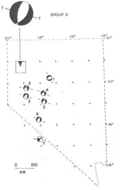
analysed by plotting the sense of motion on an upper-hemisphere stereographic projection centred on the epicentre. In this diagram compressional first arrivals are denoted by solid circles and dilations by open circles. Generally, the sense of first motion forms a pattern on the stereonet projection that can be bounded by the traces of two planes. One of these planes is the fault plane itself, and the other is an auxiliary fault plane, that is, a plane perpendicular to the actual fault plane in whose pole is the pole of motion. Because two planes are needed to form a pattern that encloses the first arrivals, ambiguity as to which one is the actual fault plane exists unless other information is available to make the selection.

The use of fault plane solutions is valuable in determining whether the earthquake activity in a prospect area is anomalous or typical of the region. An example of such an application is shown in Fig. 7, where the fault plane solution observed for earthquakes within a small prospect area shown at the top of the map is compared with earlier more general fault plane solutions in the same area. The direction of tension as indicated by the fault plane solution is the same in the prospect area as in the region, indicating that the local earthquake distribution is controlled by the same crustal phenomena.

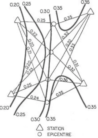
Another potentially valuable determination that can be made is that of Poisson’s ratio. Poisson’s ratio is the ratio of lateral strain to strain in the direction of stress when a cylinder of rock is subjected to uniaxial stress. Poisson’s ratio is also definable in terms of the ratio of compressional to shear wave velocities. Poisson’s ratio can be important in geothermal exploration inasmuch as it seems to be an indicator of the degree of fracturing in a rock. Both experimental and theoretical analyses have indicated that extensive fracturing of a liquid-filled rock causes Poisson’s ratio to be higher than normal. This causes a minor reduction in the p-wave velocity and a significant reduction in s-wave velocity.

Poisson’s ratio is determined from Wadati plots as described previously; that is, from plots of p – s arrival times as a function of p arrival times. Figure 8 shows a presentation of Poisson’s ratio determinations on a plane map. Each value is written along the assumed ray path from the epicentre to the receiver location, although there is no certainty that straight-line wave propagation took place. The significant anomaly in Poisson’s ratio characterised in these data corresponds to the location of a successful geothermal well that was subsequently drilled.

Fig. 8. Results of determinations of Poisson’s ratio for microseismic survey carried out on East Rift zone of Kilauea Volcano, Hawaii. Values for Poisson’s ratio are plotted along apparent straight-line travel paths from epicentre to seismograph.

earthquakes, could be used to locate large hot bodies that act as the source of geothermal systems. This technique has been the subject of considerable research in recent years, but has been faced by practical difficulties during its current deployment. Teleseisms that occur at great enough distances to be of use in p-wave delay surveys occur only rarely, perhaps a few times a month, with the magnitudes needed to obtain accurate p-wave arrival times. In order to obtain a detailed picture of subsurface structure, many hundreds of p-wave arrivals must be recorded. This can only be done by using a few stations over a long period of time or a very large number of stations for a shorter period of time. Each approach represents a relatively large investment.

Microseismicity is often not only natural but also induced by geothermal activity. One major cause appears to be injection, which results in the reservoir rock being rapidly cooled.At the Geysers geothermal field injection has increased by about 50% the number of M=2.4 events being recorded, with no increase observed in M=2.5 events.

5.2 ACTIVE SEISMIC METHODS

Both seismic reflection and seismic refraction surveys have been used in geothermal exploration. Seismic refraction surveys have been used to a limited extent because of the amount of effort required to obtain refraction profiles giving information at depths of 5 to 10 km, and the problems caused by the generally high degree of complexity of geological structures in areas likely to host geothermal systems. On the other hand, standard seismic reflection surveys have often yielded surprisingly useful results, even in areas that were expected to prove difficult. The primary requirement for using the seismic reflection technique is that the subsurface be laminar in acoustic properties so that reflectors can be traced horizontally and interruptions in reflectors can be used to identify faults where displacement has taken place.

vibrator and the geophones. Data quality can be enhanced by synchronously adding reflections that arrive from the same reflection point on a subsurface interface, but in so doing corrections must be made for the difference in travel times that is associated with the difference in separation from transmitter to receiver.

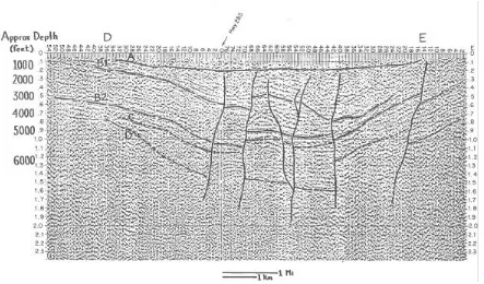
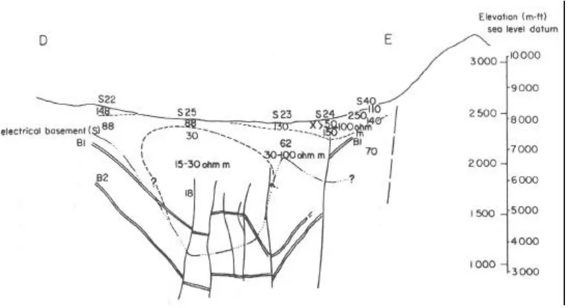
Fig. 9. Seismic reflection profile in Colorado. Events B1 and B2 are volcanic flows, C is flow bottom, D is probably Paleozoic carbonate sequence. Near-vertical lines are faults.

Fig. 10. Resistivity cross section interpreted from Schlumberger soundings along the same profile as seismic section shown in Fig. 8. Reflective horizon from Fig. 8 are shown.

Procedures for acquiring and processing seismic reflection data are well developed. Extensive computer facilities must be available to permit reduction of field observations to time sections such as are shown here, and to enhance the events that serve to trace the marker horizons in the section. An added merit of modern data processing as used in seismic reflection analysis is that, by varying the separation between vibrator and geophone spread, it is possible to determine the average acoustic wave speed to the depth of a reflector. When a series of reflectors is apparent on a seismic section, a seismic velocity profile can be extracted from the measurements. Seismic velocities themselves are useful in recognising anomalies caused by temperature in relatively shallow rocks.

6. GEOPHYSICAL WELL LOGGING AND BORE HOLE METHODS

many wells are logged, the EM tomography method may define the distribution of resistivity around the borehole and the whole area interested by drilling.

Beside well logging, the use of drill holes to place the equipment in an advantageous position to explore subsurface can be an important part of an exploration program. Instrumentation must be of small diameter, water tight and designed to operate under adverse environmental conditions.

The mise a la masse method is one of the oldest methods used in-hole and is used when a prospect hole penetrates a highly conductive zone. A current electrode is embedded in the conductive zone and energized with direct current, the other electrode being a large distance away on surface. The extent, dip, strike and continuity of the zone will be better indicated by introducing the current directly into it than by the usual mapping techniques. Lately, methods using the casing pipe itself as a charged current electrode instead of the buried point source have been used to monitor fluid flow behaviour during reinjection and during hydraulic fracturing operations in hot dry rocks.

In the cross-hole resistivity survey a trasmitter is located in one hole while a receiver is drawn up another, with the strength of the signal at the receiver being recorded. The attenuation of the signal as it travels through the medium between the holes will depend on the resistivity structure. In a general sense, attenuation will be greater if the field senses a region of low resistivity, and lower if a region of high resistivity is seen.

7. ELECTRICAL METHODS

Various methods for measuring electrical resistivity are used in geothermal exploration, based on the premiss that temperature affects the electrical properties of rocks. At the lower end of the temperature scale, up to the critical temperature for water, the effect of temperature is to enhance the conductivity of the water in the pores of the rock. In such rocks, electrical conduction takes place solely by passage of current through the fluid in the pores, since almost all rock-forming minerals are virtual insulators at these temperatures. The maximum enhancement in conductivity is approximately sevenfold between 350°C and 20°C for most electrolytes (Fig. 11).

Temperature is not the only factor affecting the conductivity of rocks. An increase in the water content or an increase in the total amount of dissolved solids can increase the conductivity by large amounts(Fig. 12). Both phenomena are sometimes associated with geothermal activity. As a result, it is not unusual to see an increase in conductivity by an order of magnitude or more in a geothermal reservoir compared with rocks at normal temperatures removed from the reservoir.

Fig. 12. Dependence of the conductivity of an electrolytic solution on the amount of salt in solution at a temperature of 18°C: for various common salts, acids and bases (left) and at various temperatures (right)

At temperatures approaching the melting point of a rock, even more significant changes in electrical properties take place. At normal temperatures for the surface of the earth, silicate minerals have very low conductivity, generally less than 10-6Ω-1m-1. As the temperature increases, so does this conductivity increase: slowly at first, and then much more rapidly at temperatures near the melting point. A typical set of curves of the conductivity plotted against the reciprocal of the absolute temperature is shown in Fig. 13. At temperatures within about 100°C of the melting point, the conductivity becomes high enough to become comparable with conductivities in water-saturated rocks.

Such high conductivities provide a target for geophysical exploration, but the very high temperatures associated with the source of a geothermal system occur at depths that are too great to be considered for exploitation. In a typical geothermal system, one would expect to find a deep anomaly in electrical conductivity associated with thermal excitation of conduction in the massive crystalline rock comprising the basement. At shallower depths in the section, one would expect to find an anomaly in electrical conductivity associated with the reservoir filled with hot geothermal fluids.

controlled-source methods are used, as well as the Schlumberger sounding method, the dipole – dipole traversing method, and the bipole–dipole mapping method. All of these techniques have as their objective the mapping of electrical structures at depths that are meaningful in terms of geothermal exploration. These depths must be several kilometres at least when looking for the anomaly in conductivity associated with reservoir rocks, and several tens of kilometres when seeking the thermally excited conductive zone associated with the source of a geothermal system.

Fig. 13. Summary of data relating electrical conductivity of dry rocks to reciprocal of the absolute temperature.

There is one main difference between electromagnetic (inductive) and resistivity techniques. The former usually provide information on conductivity-thickness products of conductive layers, whereas they usually provide only thickness information on resistive layers. On the contrary, resistivity techniques usually provide information on resistivity-thickness products for resistive layers and conductivity-resistivity-thickness products for conductive layers.

7.1 NATURAL SOURCE METHODS

7.1.1 The Magnetotelluric Method

magnetospheric currents that arise when plasma emitted from the sun interacts with the earth’s magnetic field. These currents give rise to time-varying magnetic fields in the frequency range from 0.1 Hz downwards, which are termed ultra-low frequency pulsations (ULF). ULF in turn induce eddy currents in the earth, with the eddy current density being controlled by the local conductivity structure. Superimposed onto this field are random fluctuations whose intensity vary with electrical disturbances in the ionosphere. These pulsations occur at frequencies as high as 100 kHz, although most are much lower. One source of the higher frequency current fluctuations is electric storms. Some of the thunderstorm energy is converted to electromagnetic fields, which are propagated in the ionosphere-earth interspace. These signals are called atmospherics or spherics. The configuration of the EM fields above the surface is slightly different for spherics than for ULF pulsations: the former propagate horizontally while the latter are assumed to propagate vertically. Because the very large resistivity contrast between the air and the earth, both signals behave in the same way at the surface and beneath it. They diffuse downward, the changing horizontal magnetic field inducing a changing horizontal electric field at right angles, though Faraday's law.

At large distances from the source the resulting electromagnetic field is a plane wave of variable frequency (from about 10-5 Hz up to audio range at least). The subsurface structure can be studied by making simultaneous measurements of the strength of the magnetic field variations at the surface of the earth and the strength of the electric field component at right angles in the earth. Because the direction of polarisation of the incident magnetic field is variable and not known beforehand, it is common practice to measure at least two components of the electric field and three components of the magnetic field variation to obtain a fairly complete representation. For surveys that are intended for the study of electrical structures tens of kilometres in depth, the range of frequencies needed to achieve penetration is from a few tens of Hertz to a few hundred microHertz. Inasmuch as the natural noise field is not particularly well structured, but consists of an unpredictable assemblage of impulsive waveforms, it is necessary to analyse the natural field over a time span which is long compared to the period of the lowest frequencies being studied. Thus, if the lowest frequency desired in a survey is 500 µHz (period of 2000 s), it is necessary to analyse the field over a time duration at least 10 times as great, or 20 000 s. This represents the single largest disadvantage of the magnetotelluric method: it provides slow coverage of a prospect area and is therefore costly.

In most systems for carrying out magnetotelluric surveys today, the five field components are converted to digital form and are either stored for later spectral analysis or converted immediately to spectral form before being stored. The accuracy with which the data are converted to digital form is important; a dynamic range of 16 bits is desirable so that weak spectral components will be recognisable in the presence of other, stronger spectral components. In order to obtain spectra at frequencies as high as several tens of Hertz, a maximum sampling rate of 100 Hz is required.

Once the various spectra have been calculated they must be converted to values of apparent resistivity as a function of frequency. In this reduction it is assumed that at any given frequency there is a linear relationship between the electric field vector and the magnetic field vector

where Z is the impedance of the electromagnetic field. Z is determined by resistivity structure and frequency. At each angular frequency ω, in (or at the surface of) a uniform half-space of conductivity σ

The ratio Ex/Hy at the surface (the subscripts indicates cartesian coordinates) is

particularly important, viz:

Ex/Hy = ωµ/k = (1 + i)(ωµ/2σ)1/2

Frequency will be accurately known since relative time must be precisely maintained while acquiring data. Therefore the previous equation shows directly the relationships between the measured fields and the conductivity. In particular, the ratio of Ex to Hy is proportional to (ρ)1/2, where ρ = 1/σ. Setting Ex/Hy = Zxy we get

degrees in this (uniform half-space) model. The previous equation is usually written as:

ρxy= kilometer and gammas or nanoteslas, respectively), and looking only at amplitude, then

In order to satisfy Maxwell’s equations, within the earth E and B vary as

A = A0 e-i(kz-ωt) = A0 eiωt e-iαz e-αz

where A0 is the surface value. That is, the fields vary as the product of four terms:

1. eiωt, a sinusoidal time variation,

2. e-iαz, a sinusoidal depth variation,

3. e-αz, an exponential decay with depth, and 4. A0

From the third term, the amplitudes at z = δ =1/α are 1/e of their surface values, which is why δ is called the skin depth. A plot of skin depth versus frequency and resistivity can be found in the following diagram:

A useful approximation is given by

δ≈ 500 ρ _f

In more complicated models, e.g. horizontal layers or 2-D or 3-D structures, the relations between the E and H fields also become more involved. In horizontal layers some energy is reflected at each interface, and internal reflection occurs within each layer. The expressions for E and H include two terms in each layer, of the form:

Ae+ikz + Be-ikz

right angles to one another unless there is anisotropy in the horizontal plane. We can still get Ex and Hy (or Ey and Hx) on the surface and do the resistivity calculation, but the result

depends on frequency and is now an apparent resistivityρa(f).

As a specific indication of the intuitive behavior of ρa let us consider two 2-layer cases

(Fig. 14). The top layer is the same in both models, but ρ2 = 10ρ1 in the one case and ρ2 =

(1/10) ρ1 in the other. At high frequencies such that the skin depth in the first layer is much

less than its thickness, ρa = ρ2 in both cases. As frequency decreases and skin depth

increases to the point that it is much greater than d, ρa goes to 0.1 in one case and to 10 in

the other, and stays there as frequency goes to zero. Note the small undershoot/overshoot in

ρa and Φ as frequency decreases. Also note that the phase response occurs at higher

frequencies than the apparent resistivity response. Phase is asymptotic to 45 degrees at both high and low frequencies for a finite number of uniform layers. If thickness varies but ρ1

and ρ2 are the same (Fig. 15), then frequency has to go to a lower value in the thicker layer

model for the skin depth to exceed thickness and the second layer to become important. In a three-layer model, ρa is asymptotic to ρ1 at high frequency and to ρ3 at low

frequency. In between it approaches ρ2. How close it gets depends on the thicknesses and

resistivities of both layers 1 and 2. Obviously our ability to resolve several layers depends on their resistivities and thicknesses, on the range of frequencies we record, and on the scatter in the points on the curve.

Fig. 14. MT apparent resistivity and phase responses of two-layer models. Model A – resistive basement. Model B – conductive basement.

The relationships among the field components at a single site are systematically contained in the impedance and the tipper. They are the quantities from which conductivity structure is interpreted. In general, Hx has an associated Eyand some Ex, both of which are

proportional to Hx. Likewise, Hy causes an Ex and some Ey, so that at each frequency we

would expect a linear system to behave as:

Ex= Zxy Hy + ZxxHx

Fig. 15. Changes in MT responses with layer thickness T for a two-layer model.

where each term is frequency dependent. This is commonly written as:



system is linear so that the electric fields are due only to magnetic fields, and the contributions of noise were ignored.

In practice we are often interested in regarding the fields or the tensor elements as if they had been measured in some other set of coordinate directions. For instance, the strike direction is seldom known very precisely at the time of a field survey. If we rotate the vector E field through angle +θ (clockwise as seen from above) to be E’, then:

E′x = cosθ Ex + cosθ Ey E′y = -sinθ Ex + sinθ Ey

E′ = RE.

In the same way,

H′ =RH

and

Z′ =RZRT,

where RT, the transpose of R, is

RT =

  

 −

θ θ

θ θ

cos cos

sin

sin

Starting from a tensor impedance Z which is derived from measurements, and assuming 2-D conditions, several different means have been used to find the rotation angle c between measurement direction and strike. One of these is to rotate the Zij in steps (say 5 degrees),

plot them on a polar diagram, and pick an optimum angle from the plots. An optimum angle maximizes or minimizes some combination of the Zij. These interesting diagrams,

called polar figures or impedance polar diagrams, are usually plotted at many frequencies, because in practice the strike direction often changes with depth. Fig. 16 shows such plots for a 2-D model (Zxy only).

Another way to find θ0 is to differentiate Zxy(θ) andZyx(θ) with respect to θ to give an

at each frequency. His solution

4θ0 = tan-1

[

(

)(

) (

₂

) (

₂

)

]

There is no solution in the 1-D case, whereas in a clearly 2-D case it usually has a definite value. In the 3-D case its meaning is usually questionable and there is considerable research in progress into ways to present and interpret Zij in structural terms. Of the four

values between 0 and 180 degrees, the ”choice” of strike direction is started by evaluating the mentioned optimization at two adjacent values, one a minimum and the other a maximum. This leaves four possible solutions at 90 degree intervals, or two possible strike directions. The choice between these solutions can only be made from independent information, usually the relations between vertical and horizontal H components or from geological constraints.

When the coordinates are rotated, certain combinations of terms are constant even though the individual terms vary. These are:

Zxx + Zyy = c1,

Zxy – Zyx= c2 ,

and

ZxxZyy – ZxyZyx= c3,

where the absolute value is the determinant of the impedance tensor. The ratio c1/c2 is the impedance skew. c1 will be zero in (noise-free) 1-D and 2-D models, so the skew is used as a measure of three dimensionality. It does not change with rotation of coordinates.

A quantity which does vary with setup direction is impedance ellipticity,

β(θ) =

( )

( )

along the strike. Impedance ellipticity, like impedance skew, is used to indicate whether response at a site is 3-D.

It can usually be assumed that Hz≈ 0 except near lateral conductivity changes, where ∇

× E has a vertical component. There, the relationship between Hz and the horizontal

Hz = TxHx + TyHy

where the elements Ti are complex since they may include phase shifts. Given a 2-D

structure with strike in the x′ direction, in those coordinates the previous equation simplifies to:

Hz = Ty′Hy′

Here, T ′, since it represents a tipping of the H vector out of the horizontal plane, is called the tipper. T ′ is of course zero for the 1-D case. The modulus of T ′ is rarely as great as 1, with 0.1 to 0.5 being the common range. The lower part of the range is often blurred by noise, since Hz is so weak. The required rotation angle ϕ to x′ can be estimated by the field

data by finding the horizontal direction y′ in which H(ϕ) is most highly coherent with Hz.

There is generally a definite solution in the ”almost” 2-D situation. In that case the phases of Tx and Ty are the same, the ratio Ty/Tx is a real number, and

ϕ = arctan (Ty/Tx).

Another use of the tipper, besides helping resolve ambiguity in strike, is to show which side of a contact is more conductive. Near a conductor-resistor boundary, the near-surface current density parallel to strike is larger on the conductive side. If it is looked at as a simple problem in dc magnetic fields of the excess currents, the magnetic field in the vertical plane perpendicular to the contact will ”curve around” the edge of the conductor, by Faraday’s law. Thus Hz will be directed downward when the horizontal component is

outward, and vice versa, depending on current direction. In a real situation, the phase of Hz

depends on the conductivities, frequency, and distance from the contact. However, in practice the relations can often be used to indicate the direction to a conductive region.

desirable in that the magnetotelluric method does not always provide useful results, even after measurements have been made with reliable equipment. If the natural electromagnetic field strength is unusually weak during a recording period, or if there is some phenomenon which precludes an effective analysis of the field, it may be necessary to repeat the measurements at a more favourable time. When the analysis is done in the field, decisions about re-occupying stations and siting additional stations can be made in a timely manner that will reduce overall operating costs.

The magnetotelluric method has found an application in geothermal exploration primarily because of its ability to detect the depth at which rocks become conductive because of thermal excitation. In areas of normal heat flow, this depth ranges from 50 to 500 km, but in thermal areas the depth may be 10 km or less. An example of the detection of anomalously shallow depths to conductive rocks is shown in Fig. 8, which illustrates the results of a magnetotelluric survey in the vicinity of The Geysers geothermal field, California, USA. Conductive rocks are found at depths of less than 10 km, a few miles north of the main producing part of the field.

7.1.2 The self-potential method

Self-potential or spontaneous polarization (SP in either cases) surveys are a form of electrical survey but, when self- potential surveys are carried out, only the naturally existing voltage gradients in the earth are measured, and for this reason this section appears among the natural-source methods. These natural voltages have a variety of causes, including the oxidation or reduction of various minerals by reaction with groundwater, the generation of Nernst voltages where there are concentration differences between the waters residing in various rock units, and streaming potentials, which occur when fresh waters are forced to move through a fine pore structure, stripping ions from the walls of the pores.

The self-potential method has been used in mineral exploration to find ore deposits by observing voltages generated as ore minerals oxidise. The method has also been used very extensively in borehole surveys to determine the salinity of pore fluids through the voltage generated by the Nernst effect. In geothermal areas, very large self-potential anomalies have been observed, and these are apparently caused by a combination of thermoelectric effects and streaming potentials where the temperature has caused an unusual amount of groundwater movement.

Implementation of an SP survey is straightforward. The objective is to map the electrical potential over the surface of the earth in an area where one hopes to find a source of spontaneous electric current generation. A self-potential survey is carried out by placing a pair of half-cells in contact with the ground with a separation of tens of metres to several kilometres.

Two different field procedures can be used in mapping SP: the single reference method, and the leap-frog method. In the single reference method, one non-polarizing electrode is held fixed at a reference point while the other electrode is moved about over the survey area to determine the distribution of potential over the region. This is the most straightforward method, but can map only areas of few hundred meters square becuase large separation between electrods indeces telluric alectric voltages to the SP. IN the leap-frog method the two electrodes are moved along a closed survey path. After each measurement, the trailing electrode is moved ahead of the leading electrode for the next measurement. The incremental voltages observed along the loop are succesively added and subtracted to arrive to a potential map with respect to the starting point of the loop. The net voltage when the loop closes should be zero; any residual voltage reflects survey errors and can be distributed around the loop.

In areas with strong geothermally related self-potential anomalies, variations of as much as several volts can be observed over distances that amount to a few hundred metres to a few kilometres. An example of a self-potential contour map of a thermal area in Hawaii is shown in Fig. 17.

Fig. 17. Results of a self-potential survey of a small area in Hawaii. Contour interval is 100 mV. Areas of low voltage are indicated by interior ticks on the contour. The filled circle indicates the location of a successful geothermal wildcat well.

7.2 ARTIFICIAL SOURCE ELECTROMAGNETIC METHODS

Most EM soundings consist of measurements at a number of frequencies or times using a fixed source and receiver. The distribution of currents induced in the earth depends on the product of electrical conductivity, magnetic permeability and frequency. Since low-frequency currents diffuse to greater depths than high-low-frequency currents, measurements of the EM response at several frequencies or times contain information on the variation of conductivity with depth. This technique, sometimes called parametric sounding, is similar to the natural-source EM sounding technique. Alternatively, soundings can be made by measuring the response at several source-receiver separations at a single frequency or time. In practice, this technique is employed in the frequency-domain but not in the time-domain. Frequency-domain measurements made at large source-receiver separations are influenced more by deep layers than are measurements made at small separations; hence a set of such measurements made at several spacings contains information on the variation of conductivity with depth. These soundings are often called geometric or distance soundings

and resemble geoelectrical soundings.

EM soundings methods have particular advantages and disadvantages compared with natural-source sounding methods and direct-current resistivity sounding methods. Some EM sounding methods provide better resolution and are less easily distorted by lateral variations in resistivity than soundings obtained with natural-source methods. However, for reconnaissance studies and deep soundings, controlled-source EM sounding may be more expensive than natural-source sounding. Due to power requirements, EM sounding has generally been limited to depths of a few kilometers or less whereas natural-field methods can be used to sound through the crust and into the upper mantle.

In contrast to direct-current (dc) methods, most EM methods are effective in resolving the parameters of conductive layers but are less effective in determining the resistivity of resistive layers. On the other hand, highly resistive layers do not screen deeper layers from being resolved by EM soundings as is the case with dc soundings. Most EM measurements depend only on the longitudinal conductivity of a horizontally layered earth whereas resistivity measurements depend on both transverse and longitudinal resistivity. Thus, in principle, EM soundings can yield more accurate depth estimates than dc resistivity soundings over an isotropic earth. Of course, EM soundings made with a grounded wire source and receiver give dc resistivity results at asymptotically low frequencies. The question of whether EM or resistivity soundings are least affected by lateral variations in resistivity depends on the specific techniques used in each case and on the scale of the inhomogeneity. Also the relative cost of EM and resistivity soundings depends on the technique and the application; either can be the least expensive for a particular purpose.

The source is usually an insulated loop. In the analysis of systems and interpretation of results small loops can be treated mathematically as time-varying magnetic dipoles, especially if the loop dimensions are less than five times the distance to the nearest receiver. The moment (source strength) of the dipole depends on the current as well as turns-area product of the loop.

In most frequency-domain (FEM) systems, a current having approximately a sinusoidal or a square waveform is driven through the antenna by an amplifier or switcher, and the frequency is usually changed in discrete steps. In time-domain (TEM) systems the most common waveform is a train of approximately square-bipolar pulses with an off-time between pulses.

Three types of receivers are used for EM soundings: induction coils, magnetometers and grounded wires.

In the most general case, three orthogonal components of the magnetic field and two orthogonal components of the electric field parallel to the earth's surface can be measured. Frequency-domain results are often expressed in terms of V/I, B/I, or dB/dt/I, where I is the source current, V is the voltage difference, and B is the magnetic flux density. Time-domain results are expressed as impedances, V/I. Impedance is then transformed to apparent resistivity. Apparent resistivity is defined as the resistivity of the homogeneous earth which would produce the measured response at each frequency or time.

The geometry of most dipole-dipole system can be specified by giving the orientation of the source and receiver antennas and the orientation and length of the line joining the center of the two antennas. Typical source-receiver geometries are shown in Fig. 18.

A geometric sounding may be made by leaving the source fixed and moving the receiver, or, both source and receiver may be moved with respect to the center of the array.

The range of depths which can be explored with FEM generally depends on the source-receiver separation as well as the frequency used. In FEM it is always necessary to somehow distinguish the secondary field from the primary field. The primary field is the alternating magnetic field induced by the alternating current flowing in the transmitter in the range of a few hundred Hz to a few kHz. The primary field induces an alternating current to flow in all the conductors present in the earth (eddy currents), which induces an alternating magnetic field, called secondary field, which also extends through the region which includes the receiver. The secondary field from a particular layer will be very small compared with the primary field unless the separation between the source and receiver is on the order of the depth to the layer or deeper. Thus it is generally necessary to employ source-receiver separations of the order of one or two times the maximum depth to be sounded; at a smaller separation than this it is not possible to accurately measure the small secondary field in the presence of the much larger primary field. If the spacing is too large there is difficulty resolving the parameters of thin layers, especially when they are deep. For measurements in the near zone the spacing should not be larger than five times the thickness of any layers to be resolved.

In TEM measurements a strong direct current is passed though an ungrounded loop. At time t=0 this current is abruptly interrupted. The secondary field due to the induced eddy currents in the ground are then recorded in the absence of the primary field. The depth range for TEM (made during the current off-time) depends on the sample time measured and signal-to-noise ratio, and not on the source-receiver separation; in principle one can sound to any required depth using a single small loop.

In geothermal exploration where depths of several kilometres are to be probed, in TEM the total duration of the transient process ranges from half a second to several tens of seconds, again depending on the electrical structure. In normal operating practice, the signal is enhanced by transmitting many consecutive signals, with the corresponding transient magnetic induction signals being synchronously added.

The product of a time-domain electromagnetic sounding survey is a curve relating apparent resistivity to the time following the beginning of the transient coupling between source and receiver. It is presumed that, as this time becomes progressively larger, the eddy currents giving rise to the transient coupling occur at greater and greater depths beneath the receiver. In a complete interpretation, the response observed in the field is modelled for reasonable earth structures in much the same manner as with any of the other electrical methods.

7.3 DIRECT CURRENT METHODS

The direct current resistivity method comprises a set of techniques for measuring earth resistivity that are significantly simpler in concept than the magnetotelluric method. The magnetotelluric method is an induction method in which the depth of penetration of the field is controlled by the frequency of the signals analysed. The direct current methods achieve control of the depth of the penetration by regulating the geometry of the array of equipment used.

Three principal variations of the direct current method have found use in geothermal exploration, though there has been some controversy in the literature over the relative merits of these techniques. The best tested of the techniques is the Schlumberger sounding method. With the Schlumberger array, electrodes are placed along a common line and separated by a distance, which is used to control the depth of penetration. The outer two electrodes drive current into the ground, while the inner two, located at the midpoint between the outer two, are used to detect the electric field caused by that current. The outer two electrodes are separated by progressively greater distances as a sounding survey is carried out, so that information from progressively greater depths is obtained. In a survey of a geothermal area, the spacings between electrodes will be increased incrementally from distances of a few metres or tens of metres to distances of severa1 kilometres or more.

The Schlumberger method has several limitations, including the relatively slow progress with which work can be carried forward in deep sounding, and the fact that in areas of geothermal activity the lateral dimensions of the areas of anomalous resistivity may be considerably smaller than the total spread required between electrodes.

In order to detect the presence of lateral discontinuities in resistivity, the bipole–dipole and dipole–dipole techniques have come into use. In the dipole–dipole technique, four electrodes arrayed along a common line are again used, but in this case the outer two electrodes at one end of the line provide current to the ground while the outer two electrodes at the other end of the line are used to measure the voltage caused by that current. In a survey, the receiving electrodes and transmitting electrodes are separated progressively by increments equal to the separation between one of the pairs, in the direction along which they are placed. The separation between the two dipoles can be increased from one dipole length to as much as 10 dipole lengths. When this has been done the current dipole is advanced by one dipole length along the traverse and the procedure repeated. The process is continued with the entire system moving along a profile.

As the final product, a pseudosection is compiled in which each value of apparent resistivity is plotted on a cross-section beneath the midpoint of the array with which the measurement was taken, and at a depth beneath the surface which is proportional to the separation between dipole centres. The result is a contoured section of apparent resistivity values which sometimes shows a good correlation with the actual distribution of resistivity in the earth. The dipole–dipole method has the advantage of portraying the effects of lateral changes in resistivity clearly, but suffers from the disadvantage of being a cumbersome method to apply in the field.