generatingfunctionology
Herbert S. Wilf
Department of Mathematics
University of Pennsylvania
Philadelphia, Pennsylvania
Copyright 1990 and 1994 by Academic Press, Inc. All rights re-served. This Internet Edition may be reproduced for any valid educational purpose of an institution of higher learning, in which case only the reason-able costs of reproduction may be charged. Reproduction for profit or for any commercial purposes is strictly prohibited.
Preface
This book is about generating functions and some of their uses in discrete mathematics. The subject is so vast that I have not attempted to give a comprehensive discussion. Instead I have tried only to communicate some of the main ideas.
Generating functions are a bridge between discrete mathematics, on the one hand, and continuous analysis (particularly complex variable the-ory) on the other. It is possible to study them solely as tools for solving discrete problems. As such there is much that is powerful and magical in the way generating functions give unified methods for handling such prob-lems. The reader who wished to omit the analytical parts of the subject would skip chapter 5 and portions of the earlier material.
To omit those parts of the subject, however, is like listening to a stereo broadcast of, say, Beethoven’s Ninth Symphony, using only the left audio channel.
The full beauty of the subject of generating functions emerges only from tuning in on both channels: the discrete and the continuous. See how they make the solution of difference equations into child’s play. Then see how the theory of functions of a complex variable gives, virtually by inspection, the approximate size of the solution. The interplay between the two channels is vitally important for the appreciation of the music.
In recent years there has been a vigorous trend in the direction of finding bijective proofs of combinatorial theorems. That is, if we want to prove that two sets have the same cardinality then we should be able to do it by exhibiting an explicit bijection between the sets. In many cases the fact that the two sets have the same cardinality was discovered in the first place by generating function arguments. Also, even though bijective arguments may be known, the generating function proofs may be shorter or more elegant.
The bijective proofs give one a certain satisfying feeling that one ‘re-ally’ understands why the theorem is true. The generating function argu-ments often give satisfying feelings of naturalness, and ‘oh, I could have thought of that,’ as well as usually offering the best route to finding exact or approximate formulas for the numbers in question.
This book was tested in a senior course in discrete mathematics at the University of Pennsylvania. My thanks go to the students in that course for helping me at least partially to debug the manuscript, and to a number of my colleagues who have made many helpful suggestions. Any reader who is kind enough to send me a correction will receive a then-current complete errata sheet and many thanks.
Herbert S. Wilf Philadelphia, PA September 1, 1989
This edition contains several new areas of application, in chapter 4, many new problems and solutions, a number of improvements in the pre-sentation, and corrections. It also contains an Appendix that describes some of the features of computer algebra programs that are of particular importance in the study of generating functions.
I am indebted to many people for helping to make this a better book. Bruce Sagan, in particular, made many helpful suggestions as a result of a test run in his classroom. Many readers took up my offer (which is now repeated) to supply a current errata sheet and my thanks in return for any errors discovered.
Herbert S. Wilf Philadelphia, PA May 21, 1992
CONTENTS
Chapter 1: Introductory Ideas and Examples
1.1 An easy two term recurrence . . . 3
1.2 A slightly harder two term recurrence . . . 5
1.3 A three term recurrence . . . 8
1.4 A three term boundary value problem . . . 10
1.5 Two independent variables . . . 11
1.6 Another 2-variable case . . . 16
Exercises . . . 24
Chapter 2: Series 2.1 Formal power series . . . 30
2.2 The calculus of formal ordinary power series generating functions 33 2.3 The calculus of formal exponential generating functions . . . . 39
2.4 Power series, analytic theory . . . 46
2.5 Some useful power series . . . 52
2.6 Dirichlet series, formal theory . . . 56
Exercises . . . 65
Chapter 3: Cards, Decks, and Hands: The Exponential Formula 3.1 Introduction . . . 73
3.2 Definitions and a question . . . 74
3.3 Examples of exponential families . . . 76
3.4 The main counting theorems . . . 78
3.5 Permutations and their cycles . . . 81
3.6 Set partitions . . . 83
3.7 A subclass of permutations . . . 84
3.8 Involutions, etc. . . 84
3.9 2-regular graphs . . . 85
3.10 Counting connected graphs . . . 86
3.11 Counting labeled bipartite graphs . . . 87
3.12 Counting labeled trees . . . 89
3.13 Exponential families and polynomials of ‘binomial type.’ . . . . 91
3.14 Unlabeled cards and hands . . . 92
3.15 The money changing problem . . . 96
3.16 Partitions of integers . . . 100
3.17 Rooted trees and forests . . . 102
3.18 Historical notes . . . 103
Exercises . . . 104
4.1 Generating functions find averages, etc. . . 108
4.2 A generatingfunctionological view of the sieve method . . . 110
4.3 The ‘Snake Oil’ method for easier combinatorial identities . . . 118
4.4 WZ pairs prove harder identities . . . 130
4.5 Generating functions and unimodality, convexity, etc. . . 136
4.6 Generating functions prove congruences . . . 140
4.7 The cycle index of the symmetric group . . . 141
4.8 How many permutations have square roots? . . . 146
4.9 Counting polyominoes . . . 150
4.10 Exact covering sequences . . . 154
Exercises . . . 157
Chapter 5: Analytic and asymptotic methods 5.1 The Lagrange Inversion Formula . . . 167
5.2 Analyticity and asymptotics (I): Poles . . . 171
5.3 Analyticity and asymptotics (II): Algebraic singularities . . . . 177
5.4 Analyticity and asymptotics (III): Hayman’s method . . . 181
Exercises . . . 188
Appendix: Using MapleTM and MathematicaTM . . . 192
Solutions . . . 197
References . . . 224
Chapter 1
Introductory ideas and examples
A generating function is a clothesline on which we hang up a sequence of numbers for display.
What that means is this: suppose we have a problem whose answer is a sequence of numbers,a0, a1, a2, . . .. We want to ‘know’ what the sequence is. What kind of an answer might we expect?
A simple formula foran would be the best that could be hoped for. If
we find thatan=n2+ 3 for eachn= 0,1,2, . . ., then there’s no doubt that we have ‘answered’ the question.
But what if there isn’t any simple formula for the members of the unknown sequence? After all, some sequences are complicated. To take just one hair-raising example, suppose the unknown sequence is 2, 3, 5, 7, 11, 13, 17, 19, . . ., where an is the nth prime number. Well then, it would
be just plain unreasonable to expect any kind of a simple formula.
Generating functions add another string to your bow. Although giv-ing a simple formula for the members of the sequence may be out of the question, we might be able to give a simple formula forthe sum of a power series, whose coefficients are the sequence that we’re looking for.
For instance, suppose we want the Fibonacci numbers F0, F1, F2, . . ., and what we know about them is that they satisfy the recurrence relation
Fn+1 =Fn+Fn−1 (n≥1;F0 = 0; F1 = 1).
The sequence begins with 0, 1, 1, 2, 3, 5, 8, 13, 21, 34, 55, . . . There are exact, not-very-complicated formulas forFn, as we will see later, in example
2 of this chapter. But, just to get across the idea of a generating function, here is how a generatingfunctionologist might answer the question: the
nth Fibonacci number, Fn, is the coefficient of xn in the expansion of the
function x/(1−x−x2) as a power series about the origin.
You may concede that this is a kind of answer, but it leaves a certain unsatisfied feeling. It isn’t really an answer, you might say, because we don’t have that explicit formula. Is it a goodanswer?
In this book we hope to convince you that answers like this one are often spectacularly good, in that they are themselves elegant, they allow you to do almost anything you’d like to do with your sequence, and gener-ating functions can be simple and easy to handle even in cases where exact formulas might be stupendously complicated.
Here are some of the things that you’ll often be able to do with gener-ating function answers:
(a) Find an exact formula for the members of your sequence.
Not always. Not always in a pleasant way, if your sequence is
complicated. But at least you’ll have a good shot at finding such a formula.
(b) Find a recurrence formula. Most often generating functions arise from recurrence formulas. Sometimes, however, from the generating function you will find a new recurrence formula, not the one you started with, that gives new insights into the nature of your sequence.
(c) Find averages and other statistical properties of your se-quence. Generating functions can give stunningly quick deriva-tions of various probabilistic aspects of the problem that is repre-sented by your unknown sequence.
(d) Find asymptotic formulas for your sequence. Some of the deepest and most powerful applications of the theory lie here. Typically, one is dealing with a very difficult sequence, and instead of looking for anexactformula, which might be out of the question, we look for an approximate formula. While we would not expect, for example, to find an exact formula for the nth prime number, it is a beautiful fact (the ‘Prime Number Theorem’) that the nth prime isapproximatelynlognwhennis large, in a certain precise sense. In chapter 5 we will discuss asymptotic problems.
(e) Prove unimodality, convexity, etc. A sequence is called uni-modal if it increases steadily at first, and then decreases steadily. Many combinatorial sequences are unimodal, and a variety of methods are available for proving such theorems. Generating func-tions can help. There are methods by which the analytic proper-ties of the generating function can be translated into conclusions about the rises and falls of the sequence of coefficients. When the method of generating functions works, it is often the simplest method known.
(f) Prove identities. Many, many identities are known, in combina-torics and elsewhere in mathematics. The identities that we refer to are those in which a certain formula is asserted to be equal to another formula for stated values of the free variable(s). For example, it is well known that
n
X
j=0
µ
n j
¶2
=
µ
2n n
(n= 0,1,2, . . .).
1.1 An easy two term recurrence 3
obvious, but it is quite remarkable how much simpler and more transparent many of the derivations become when seen from the point of view of the black belt generatingfunctionologist. The ‘Snake Oil’ method that we present in section 4.3, below, explores some of these vistas. The method of rational functions, in section 4.4, is new, and does more and harder problems of this kind. (g) Other. Is there something else you would like to know about
your sequence? A generating function may offer hope. One ex-ample might be the discovery of congruence relations. Another possibility is that your generating function may bear a striking resemblance to some other known generating function, and that may lead you to the discovery that your problem is closely related to another one, which you never suspected before. It is noteworthy that in this way you may find out that the answer to your prob-lem is simply related to the answer to another probprob-lem, without knowing formulas for the answers to either one of the problems!
In the rest of this chapter we are going to give a number of examples of problems that can be profitably thought about from the point of view of generating functions. We hope that after studying these examples the reader will be at least partly convinced of the power of the method, as well as of the beauty of the unified approach.
1.1 An easy two term recurrence
A certain sequence of numbersa0, a1, . . . satisfies the conditions
an+1 = 2an+ 1 (n≥0;a0 = 0). (1.1.1)
Find the sequence.
First try computing a few members of the sequence to see what they look like. It begins with 0, 1, 3, 7, 15, 31, . . . These numbers look sus-piciously like 1 less than the powers of 2. So we could conjecture that
an = 2n −1 (n ≥ 0), and prove it quickly, by induction based on the
recurrence (1.1.1).
But this is a book about generating functions, so let’s forget all of that, pretend we didn’t spot the formula, and use the generating function method. Hence, instead of finding the sequence {an}, let’s find the
gener-ating function A(x) = P
n≥0anxn. Once we know what that function is, we will be able to read off the explicit formula for the an’s by expanding A(x) in a series.
To find A(x), multiply both sides of the recurrence relation (1.1.1) by
If we do this first to the left side of (1.1.1), there resultsP
n≥0an+1xn. How can we relate this to A(x)? It is almost the same as A(x). But the subscript of the ‘a’ in each term is 1 unit larger than the power ofx. But, clearly,
X
n≥0
an+1xn =a1+a2x+a3x2+a4x3+· · ·
={(a0+a1x+a2x2+a3x3+· · ·)−a0}/x =A(x)/x
since a0 = 0 in this problem. Hence the result of so operating on the left side of (1.1.1) is A(x)/x.
Next do the right side of (1.1.1). Multiply it by xn and sum over all
n≥0. The result is
X
n≥0
(2an+ 1)xn= 2A(x) +X
n≥0
xn
= 2A(x) + 1 1−x,
wherein we have used the familiar geometric series evaluation P
n≥0xn = 1/(1−x), which is valid for |x|<1.
If we equate the results of operating on the two sides of (1.1.1), we find that
A(x)
x = 2A(x) +
1 1−x,
which is trivial to solve for the unknown generating function A(x), in the form
A(x) = x
(1−x)(1−2x).
This is the generating function for the problem. The unknown numbers
an are arranged neatly on this clothesline: an is the coefficient ofxn in the
series expansion of the above A(x).
Suppose we want to find an explicit formula for the an’s. Then we
would have to expand A(x) in a series. That isn’t hard in this example, since the partial fraction expansion is
x
(1−x)(1−2x) =x
½
2 1−2x −
1 1−x
¾
={2x+ 22x2+ 23x3+ 24x4+· · ·}
− {x+x2+x3+x4+· · ·}
= (2−1)x+ (22−1)x2+ (23−1)x3+ (24−1)x4+· · ·
It is now clear that the coefficient ofxn, i.e. a
1.2 A slightly harder two term recurrence 5
In this example, the heavy machinery wasn’t needed because we knew the answer almost immediately, by inspection. The impressive thing about generatingfunctionology is that even though the problems can get a lot harder than this one, the method stays very much the same as it was here, so the same heavy machinery may produce answers in cases where answers are not a bit obvious.
1.2 A slightly harder two term recurrence
A certain sequence of numbersa0, a1, . . . satisfies the conditions
an+1= 2an+n (n≥0;a0 = 1). (1.2.1) Find the sequence.
As before, we might calculate the first several members of the sequence, to get 1, 2, 5, 12, 27, 58, 121, . . . A general formula does not seem to be immediately in evidence in this case, so we use the method of generating functions. That means that instead of looking for the sequence a0, a1, . . ., we will look for the function A(x) = P
j≥0ajxj. Once we have found the function, the sequence will be identifiable as the sequence of power series coefficients of the function.*
As in example 1, the first step is to make sure that the recurrence relation that we are trying to solve comes equipped with a clear indication of the range of values of the subscript for which it is valid. In this case, the recurrence (1.2.1) is clearly labeled in the parenthetical comment as being valid forn= 0,1,2, . . .Don’t settle for a recurrence that has an unqualified free variable.
The next step is to define the generating function that you will look for. In this case, since we are looking for a sequence a0, a1, a2, . . . one natural choice would be the function A(x) =P
j≥0ajxj that we mentioned above. Next, take the recurrence relation (1.2.1), multiply both sides of it by
xn, and sum over all the values of n for which the relation is valid, which,
in this case, means sum fromn= 0 to∞. Try to express the result of doing that in terms of the function A(x) that you have just defined.
If we do that to the left side of (1.2.1), the result is
a1+a2x+a3x2+a4x3 +· · ·= (A(x)−a0)/x = (A(x)−1)/x.
So much for the left side. What happens if we multiply the right side of (1.2.1) by xn and sum over nonnegative integers n? Evidently the result is 2A(x) +P
n≥0nxn. We need to identify the series
X
n≥0
nxn =x+ 2x2+ 3x3+ 4x4 +· · ·
There are two ways to proceed: (a) look it up (b) work it out. To work it out we use the following stunt, which seems artificial if you haven’t seen it before, but after using it 4993 times it will seem quite routine:
X
n≥0
nxn =X
n≥0
x( d
dx)x
n =x( d dx)
X
n≥0
xn =x( d
dx)
1 1−x =
x
(1−x)2. (1.2.2) In other words, the series that we are interested in is essentially the derivative of the geometric series, so its sum is essentially the derivative of the sum of the geometric series. This raises some nettlesome questions, which we will mention here and deal with later. For what values of x is (1.2.2) valid? The geometric series converges only for |x| < 1, so the ana-lytic manipulation of functions in (1.2.2) is legal only for thosex. However, often the analytic nature of the generating function doesn’t interest us; we love it only for its role as a clothesline on which our sequence is hanging out to dry. In such cases we can think of a generating function as only a formal power series, i.e., as an algebraic object rather than as an analytic one. Then (1.2.2) would be valid as an identity in the ring of formal power series, which we will discuss later, and the variable x wouldn’t need to be qualified at all.
Anyway, the result of multiplying the right hand side of (1.2.1) byxn
and summing over n≥0 is 2A(x) +x/(1−x)2, and if we equate this with our earlier result from the left side of (1.2.1), we find that
(A(x)−1)
x = 2A(x) + x
(1−x)2, (1.2.3)
and we’re ready for the easy part, which is to solve (1.2.3) for the unknown
A(x), getting
A(x) = 1−2x+ 2x 2
(1−x)2(1−2x). (1.2.4) Exactly what have we learned? The original problem was to ‘find’ the numbers {an} that are determined by the recurrence (1.2.1). We have, in
a certain sense, ‘found’ them: the number an is the coefficient of xn in the
power series expansion of the function (1.2.4).
This is the end of the ‘find-the-generating-function’ part of the method. We have it. What we do with it depends on exactly why we wanted to know the solution of (1.2.1) in the first place.
Suppose, for example, that we want an exact, simple formula for the membersanof the unknown sequence. Then the method of partial fractions will work here, just as it did in the first example, but its application is now a little bit trickier. Let’s try it and see.
1.2 A slightly harder two term recurrence 7
form
1−2x+ 2x2
(1−x)2(1−2x) =
A
(1−x)2 +
B
1−x + C
1−2x, (1.2.5)
and the only problem is how to find the constantsA, B, C.
Here’s the quick way. First multiply both sides of (1.2.5) by (1−x)2, and then letx= 1. The instant result is that A=−1 (don’t take my word for it, try it for yourself!). Next multiply (1.2.5) through by 1−2x and let x = 1/2. The instant result is that C = 2. The hard one to find is B, so let’s do that one by cheating. Since we know that (1.2.5) is an identity, i.e., is true for all values of x, let’s choose an easy value of x, say x = 0, and substitute that value of x into (1.2.5). Since we now know A and C, we find at once that B= 0.
We return now to (1.2.5) and insert the values ofA, B, C that we just found. The result is the relation
A(x) = 1−2x+ 2x 2 (1−x)2(1−2x) =
(−1) (1−x)2 +
2
1−2x. (1.2.6)
What we are trying to do is to find an explicit formula for the coefficient of xn in the left side of (1.2.6). We are trading that in for two easier
problems, namely finding the coefficient of xn in each of the summands on the right side of (1.2.6). Why are they easier? The term 2/(1−2x), for instance, expands as a geometric series. The coefficient of xn there is just 2·2n = 2n+1. The series (−1)/(1−x)2 was handled in (1.2.2) above, and its coefficient of xn is−(n+ 1). If we combine these results we see that our unknown sequence is
an = 2n+1−n−1 (n= 0,1,2, . . .).
Having done all of that work, it’s time to confess that there are better ways to deal with recurrences of the type (1.2.1), without using generating functions.* However, the problem remains a good example of how gener-ating functions can be used, and it underlines the fact that a single unified method can replace a lot of individual special techniques in problems about sequences. Anyway, it won’t be long before we’re into some problems that essentially cannot be handled without generating functions.
It’s time to introduce some notation that will save a lot of words in the sequel.
Definition. Let f(x) be a series in powers of x. Then by the symbol
[xn]f(x) we will mean the coefficient of xn in the series f(x).
Here are some examples of the use of this notation.
[xn]ex = 1/n!; [tr]{1/(1−3t)}= 3r; [um](1 +u)s=
µ
s m
.
A perfectly obvious property of this symbol, that we will use repeatedly, is
[xn]{xaf(x)}= [xn−a]f(x). (1.2.7)
Another property of this symbol is the convention that if β is any real number, then
[βxn]f(x) = (1/β)[xn]f(x), (1.2.8)
so, for instance, [xn/n!]ex = 1 for all n≥0.
Before we move on to the next example, here is a summary of the method of generating functions as we have used it so far.
THE METHOD
Given: a recurrence formula that is to be solved by the method of generating functions.
1. Make sure that the set of values of the free variable (say n) for which the given recurrence relation is true, is clearly delineated. 2. Give a name to the generating function that you will look for, and
write out that function in terms of the unknown sequence (e.g., call it A(x), and define it to be P
n≥0anxn).
3. Multiply both sides of the recurrence by xn, and sum over all values of nfor which the recurrence holds.
4. Express both sides of the resulting equation explicitly in terms of your generating function A(x).
5. Solve the resulting equation for the unknown generating function
A(x).
6. If you want an exact formula for the sequence that is defined by the given recurrence relation, then attempt to get such a formula by expanding A(x) into a power series by any method you can think of. In particular, if A(x) is a rational function (quotient of two polynomials), then success will result from expanding in partial fractions and then handling each of the resulting terms separately.
1.3 A three term recurrence
Now let’s do the Fibonacci recurrence
Fn+1 =Fn+Fn−1. (n≥1;F0 = 0; F1 = 1). (1.3.1)
Following ‘The Method,’ we will solve for the generating function
F(x) =X
n≥0
1.3 A three term recurrence 9
and on the right side we find
{F1x+F2x2+F3x3+· · ·}+{F0x+F1x2+F2x3+· · ·}={F(x)}+{xF(x)}.
(Important: Try to do the above yourself, without peeking, and see if you get the same answer.) It follows that (F −x)/x= F +xF, and therefore that the unknown generating function is now known, and it is
F(x) = x 1−x−x2.
Now we will find some formulas for the Fibonacci numbers by expand-ing x/(1−x−x2) in partial fractions. The success of the partial fraction method is greatly enhanced by having only linear (first degree) factors in the denominator, whereas what we now have is a quadratic factor. So let’s factor it further. We find that
1−x−x2 = (1−xr+)(1−xr−) (r± = (1±
thanks to the magic of the geometric series. It is easy to pick out the coefficient of xn and find
Fn =
as an explicit formula for the Fibonacci numbers Fn.
This example offers us a chance to edge a little further into what gen-erating functions can tell us about sequences, in that we can get not only the exact answer, but also an approximate answer, valid when n is large. Indeed, when n is large, since r+ > 1 and |r−| < 1, the second term in
(1.3.3) will be minuscule compared to the first, so an extremely good ap-proximation to Fn will be
But, you may ask, why would anyone want an approximate formula when an exact one is available? One answer, of course, is that sometimes exact answers are fearfully complicated, and approximate ones are more revealing. Even in this case, where the exact answer isn’t very complex, we can still learn something from the approximation. The reader should take a few moments to verify that, by neglecting the second term in (1.3.3), we neglect a quantity that is never as large as 0.5 in magnitude, and conse-quently not only is Fn approximately given by (1.3.4), it is exactly equal
to the integer nearest to the right side of (1.3.4). Thus consideration of an approximate formula has found us a simpler exact formula!
1.4 A three term boundary value problem
This example will differ from the previous ones in that the recurrence relation involved does not permit the direct calculation of the members of the sequence, although it does determine the sequence uniquely. The situation is similar to the following: suppose we imagine the Fibonacci re-currence, together with the additional dataF0 = 1 andF735= 1. Well then, the sequence{Fn}would be uniquely determined, but you wouldn’t be able to compute it directly by recurrence because you would not be in possession of the two consecutive values that are needed to get the recurrence started. We will consider a slightly more general situation. It consists of the recurrence
aun+1+bun+cun−1 =dn (n= 1,2, . . . , N −1;u0 =uN = 0) (1.4.1)
where the positive integerN, the constantsa,b,cand the sequence{dn}Nn=1−1 are given in advance. The equations (1.4.1) determine the sequence {ui}N0 uniquely, as we will see, and the method of generating functions gives us a powerful way to attack such boundary value problems as this, which arise in numerous applications, such as the theory of interpolation by spline func-tions.
To begin with, we will define two generating functions. One of them is our unknownU(x) =PN
j=0ujxj, and the second one isD(x) =
PN−1
j=1 djxj, and it is regarded as a known function (did we omit any given values of the
dj’s, like d0? or dN? Why?).
Next, following the usual recipe, we multiply the recurrence (1.4.1) by
xn and sum over the values of n for which the recurrence is true, which in this case means that we sum from n= 1 to N −1. This yields
a N−1
X
n=1
un+1xn+b
N−1
X
n=1
unxn+c N−1
X
n=1
un−1xn =
N−1
X
n=1
dnxn.
If we now express this equation in terms of our previously defined generating functions, it takes the form
a
x{U(x)−u1x}+bU(x) +cx{U(x)−uN−1x N−1
1.4 A three term boundary value problem 11
Next, with only a nagging doubt because u1 and uN−1 are unknown, we press on with the recipe, whose next step asks us to solve (1.4.2) for the unknown generating function U(x). Now that isn’t too hard, and we find at once that
{a+bx+cx2}U(x) =x{D(x) +au1+cuN−1xN}. (1.4.3)
The unknown generating function U(x) is now known except for the two still-unknown constantsu1 anduN−1, but (1.4.3) suggests a way to find
them, too. There are two values of x, call them r+ and r−, at which the
quadratic polynomial on the left side of (1.4.3) vanishes. Let us suppose that rN
+ 6= rN−, for the moment. If we let x = r+ in (1.4.3), we obtain one equation in the two unknowns u1, uN−1, and if we let x =r−, we get
another. The two equations are
au1+ (cr+N)uN−1 =−D(r+)
au1+ (cr−N)uN−1 =−D(r−).
(1.4.4)
Once these have been solved for u1 and uN−1, equation (1.4.3) then gives
U(x) quite explicitly and completely. We leave the exceptional case where
rN
+ =r−N to the reader.
Here is an application∗ of these results to the theory of spline interpo-lation.
Suppose we are given a table of values y0, y1, . . . , yn of some function y(x), at a set of equally spaced pointsti =t0+ih(0≤i≤n). We want to construct a smooth functionS(x) that fits the data, subject to the following conditions:
(i) Within each interval (ti, ti+1) (i= 0, . . . , n−1) our functionS(x) is to be a cubic polynomial (a different one in each interval!);
(ii) The functions S(x), S′(x) and S′′(x) are to be continuous on the
whole interval [t0, tn]; (iii) S(ti) =yi fori = 0, . . . , n.
A functionS(x) that satisfies these conditions is called acubic spline. Suppose our unknown splineS(x) is given byS0(x), if x∈[t0, t1], S1(x), if
x∈[t1, t2],. . ., Sn−1(x), if x∈[tn−1, tn], and we want now to determine all of the cubic polynomialsS0, . . . , Sn−1. To do this we have 2ninterpolatory conditions
Si−1(ti) =yi =Si(ti) (i= 1, . . . , n−1); S0(t0) =y0; Sn−1(tn) =yn
(1.4.5) along with 2n−2 continuity conditions
S′i−1(ti) =Si′(ti); Si′′−1(ti) =Si′′(ti) (i= 1, . . . , n−1). (1.4.6)
∗ This application is somewhat specialized, and may be omitted at a first
There are altogether 4n−2 conditions to satisfy. We haven cubic polyno-mials to be determined, each of which has 4 coefficients, for a total of 4n
unknown parameters. Since the conditions are linear, such a spline S(x) surely exists and we can expect it to have two free parameters. It is con-ventional to choose these so that S(x) has a point of inflection at t0 and at
tn.
Now here is the solution. The functions Si(x) are given by
Si(x) =
1 6h
¡
zi(ti+1−x)3+zi+1(x−ti)3+ (6yi+1−h2zi+1)(x−ti)
+ (6yi−h2zi)(ti+1−x)
¢
(i = 0,1, . . . , n−1),
(1.4.7) provided that the numbers z1, . . . , zn−1 satisfy the simultaneous equations
zi−1+ 4zi+zi+1 = 6
h2(yi+1−2yi+yi−1) (i= 1,2, . . . , n−1) (1.4.8)
in which z0 = zn = 0. It is easy to check this, by substituting x =ti and x = ti+1 into (1.4.7) to verify that (1.4.5) and (1.4.6) are satisfied. Hence it remains only to solve the equations (1.4.8).
The system of equations (1.4.8) is of the form (1.4.1), hence we can find the solutions from (1.4.3), (1.4.4). To do this, begin with the given set of points {(ti, yi)}ni=0, through which we wish to interpolate. Use them to write down
D(x) = 6
h2
n−1
X
i=1
(yi+1−2yi+yi−1)xi. (1.4.9)
Since (a, b, c) = (1,4,1) in this example, we have r± =−2±√3. Now our unknown generating function U(x) is given by (1.4.3), which reads as
U(x) = x(D(x) +z1+zn−1x
n)
(1 + 4x+x2) , (1.4.10)
in which the unknown numbersz1, zn−1 are determined by the requirement that the right side of (1.4.10) be a polynomial, or equivalently by the two equations (1.4.4), which become
z1+ (
√
3−2)nzn−1 =−D(
√
3−2)
z1+ (−
√
3−2)nzn−1 =−D(−
√
3−2). (1.4.11)
When we know U(x), which is, after all, Pn−1
1.4 A three term boundary value problem 13
Example.
Now let’s try an example with real live numbers in it. Suppose we are trying to fit the powers of 2 by a cubic spline on the interval [0,5]. Our input data are yi = 2i for i = 0,1, . . . ,5, h = 1, and n = 5. From (1.4.9)
we find that D(x) = 6x(1 + 2x+ 4x2+ 8x3). Then we solve (1.4.11) to find that z1 = 204/209 and z4 = 2370/209. Next (1.4.10) tells us that
U(x) = 204x 209 +
438x2 209 +
552x3 209 +
2370x4 209 ,
and now we know all of the zi’s. Finally, (1.4.7) tells us the exact cubic polynomials that form the spline. For example, S0(x), which lives on the subinterval [0,1], is
S0(x) = 1 + 175 209x+
34 209x
3.
Note that S0(0) = 1 and S0(1) = 2, so it correctly fits the data at the endpoints of its subinterval, and that S0′′(0) = 0, so the fit will have an inflection point at the origin. The reader is invited to find all of the Si(x)
(i= 0,1, . . . ,5), in this example, and check that they smoothly fit into each other at the points 1,2,3,4, in the sense that the functions and their first two derivatives are continuous.
One reason why you might like to fit some numerical data with a spline is because you want to integrate the function that the data represent. Integration of (1.4.7) from ti =ihto ti+1 = (i+ 1)h shows that
Z ti+1
ti
Si(x)dx= h
2(yi+yi+1)−
h3
24(zi+zi+1). (1.4.12)
Thus, fitting some data by a spline and integrating the spline amounts to numerical integration by the trapezoidal rule with a third order correction term. If we sum (1.4.12) overi= 0, . . . , n−1 we get for the overall integral,
Z nh
0
S(x)dx= trap− h
12(y0−y1−yn−1+yn)−
h3
72(z1+zn−1) (1.4.13)
in which ‘trap’ is the trapezoidal rule, and z1, zn−1 satisfy (1.4.11).
1.5 Two independent variables
In this section we will see how generating functions can be helpful in problems that involve functions of two discrete variables. We will use the opportunity also to introduce the binomial coefficients, since they are surely one of the most important combinatorial counting sequences.
Let n and k be integers such that 0 ≤ k ≤ n. In how many ways can we choose a subset of k objects from the set {1,2, . . . , n}? Let’s pretend that we don’t know how this will turn out, and allow generating functions to help us find the answer.
Suppose f(n, k) is the answer to the question. We imagine that the collection of all possible subsets of k of these n objects are in front of us, and we will divide them into two piles. In the first pile we put all of those subsets that do contain the object ‘n’, and into the second pile we put all subsets that do not contain ‘n’. The first of these piles obviously contains
f(n−1, k−1) subsets. The second pile contains f(n−1, k) subsets. The two piles together originally contained f(n, k) subsets. So it must be that our unknown numbersf(n, k) satisfy the recurrence
f(n, k) =f(n−1, k) +f(n−1, k−1) (f(n,0) = 1). (1.5.1)
To find formulas for these numbers we use (what else?) generating functions. For each n= 0,1,2, . . . define the generating function
Bn(x) =X
k≥0
f(n, k)xk.
Now multiply (1.5.1) throughout by xk and sum over k ≥1. The result is that Bn(x)−1 = (Bn−1(x)−1) +xBn−1(x), for n ≥ 1, with B0(x) = 1. Hence
Bn(x) = (1 +x)Bn−1(x) (n≥1; B0(x) = 1). (1.5.2)
Thus Bn(x) = (1 +x)n, for all n ≥ 0. Our unknown number f(n, k)
is revealed to be the coefficient of xk in the polynomial (1 +x)n. To find
a formula for f(n, k) we might, for example, use Taylor’s formula, which would tell us that f(n, k) is the kth derivative of (1 +x)n, evaluated at x = 0, all divided by k!. The differentiation is simple to do. Indeed, the
kth derivative of (1 +x)n is n(n−1)· · ·(n−k+ 1)(1 +x)n−k. If we put x = 0 and divide by k! we quickly discover that f(n, k), the number of
k-subsets of n things, is given by
n k
= n!
k!(n−k)! =
n(n−1)(n−2)· · ·(n−k+ 1)
k! (1.5.3)
1.5 Two independent variables 15
That pretty well takes care of the binomial coefficients ¡n
k
¢
when 0 ≤
k ≤ n and n, k are integers. When k is a negative integer the binomial coefficient ¡n
k
¢
= 0.
Although the second member of equation (1.5.3) is difficult to decipher if n is not a nonnegative integer, the third member isn’t a bit hard to understand, even if n is a complex number, so long as k is a nonnegative integer. So that gives us an extension of the definition of the binomial coefficients to arbitrary complex numbers n, namely,
µ
remains valid for all complex numbers n: the series terminates if n is a nonnegative integer, and it converges for |x|<1 in any case.
What is the support of ¡n
= 0? First, k must be a nonnegative integer. If n is not a nonnegative integer then ¡n
k
¢
is surely nonzero, by (1.5.4). If n is a nonnegative integer then (1.5.4) shows that ¡n
k
¢
6
= 0 iff 0 ≤ k ≤ n (in accordance with the combinatorial definition!).
A very important consequence of these facts is that ifnis a nonnegative integer, instead of writing something like Pn
k=0
xk, because the binomial coefficients vanish on all of the seemingly extra values ofk that appear in the second form of the sum. The binomial coefficients “cut off” the sum by themselves, so there is no need to do it again with the range of summation.
That being the case, we introduce two conventions that we will adhere to throughout the book.
Convention 1. When the range of a variable that is being summed over is not specified, it is to be understood that the range of summation is from −∞ to +∞.
Convention 2. When the range of a free variable in an equation is not specified, it is to be understood that the equation holds for all integer values of that variable.
For example, we will write P
k
¡n
k
¢
xk = (1 +x)n. These conventions
Let’s look at generating functions of some other kinds. If we multiply
For another exercise, let’s evaluate, for nonnegative integer k, the sum
P
n
¡n
k
¢
yn. Note that the index n runs over all integers, but that the
sum-mand vanishes unless n≥k. That sum is clearly
[xk]X
For future reference we will place side-by-side these two power series gen-erating functions of the binomial coefficients:
X
This example will have a stronger combinatorial flavor than the pre-ceding ones. It concerns the partitions of a set. By a partition of a set S
we will mean a collection of nonempty, pairwise disjoint sets whose union is
S. Another name for a partition of S is an equivalence relation on S. The sets into which S is partitioned are called theclasses of the partition.
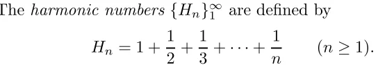
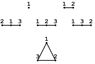
For instance, we can partition [5]∗ in several ways. One of them is as
{123}{4}{5}. In this partition there are three classes, one of which contains 1 and 2 and 3, another of which contains only 4, while the other contains only 5. No significance attaches to the order of the elements within the classes, nor to the order of the classes. All that matters is ‘who is together and who is apart.’
Here is a list of all of the partitions of [4] into 2 classes:
{12}{34}; {13}{24}; {14}{23}; {123}{4}; {124}{3}; {134}{2}; {1}{234}.
(1.6.1) There are exactly 7 partitions of [4] into 2 classes.
The problem that we will address in this example is to discover how many partitions of [n] intok classes there are. Let©n
k
ª
denote this number.
1.6 Another 2-variable case. 17
It is called the Stirling number of the second kind. Our list above shows that ©4
2
ª
= 7.
To find out more about these numbers we will follow the method of generating functions. First we will find a recurrence relation, then a few generating functions, then some exact formulas, etc.
We begin with a recurrence formula for ©n
k
ª
, and the derivation will be quite similar to the one used in the previous example.
Let positive integersn, k be given. Imagine that in front of you is the collection of all possible partitions of [n] into k classes. There are exactly
©n
k
ª
of them. As in the binomial coefficient example, we will carve up this collection into two piles; into the first pile go all of those partitions of [n] into k classes in which the letter n lives in a class all by itself. Into the second pile go all other partitions, i.e., those in which the highest letter n
lives in a class with other letters.
The question is, how many partitions are there in each of these two piles (expressed in terms of the Stirling numbers)?
Consider the first pile. There, every partition hasnliving alone. Imag-ine marching through that pile and erasing the class ‘(n)’ that appears in every single partition in the pile. If that were done, then what would re-main after the erasures is exactly the complete collection of all partitions of [n−1] intok−1 classes. There are ©n−1
k−1
ª
of these, so there must have been ©n−1
k−1
ª
partitions in the first pile.
That was the easy one, but now consider the second pile. There the letter n always lives in a class with other letters. Therefore, if we march through that pile and erase the letternwherever it appears, we won’t affect the numbers of classes; we’ll still be looking at partitions with k classes. After erasing the letter nfrom everything, our pile now contains partitions ofn−1 letters intok classes. However, each one of these partitions appears not just once, but several times.
For example, in the list (1.6.1), the second pile contains the partitions
{12}{34}; {13}{24}; {14}{23}; {124}{3}; {134}{2}; {1}{234}, (1.6.2)
and after we delete ‘4’ from every one of them we get the list
{12}{3}; {13}{2}; {1}{23}; {12}{3}; {13}{2}; {1}{23}.
What we are looking at is the list of all partitions of [3] into 2 classes, where each partition has been written down twice. Hence this list contains exactly 2©3
2
ª
partitions.
In the general case, after erasingn from everything in the second pile, we will be looking at the list of all partitions of [n−1] intok classes, where every such partition will have been written down k times. Hence that list will contain exactly k©n−1
k
ª
Therefore the second pile must have also contained k©n−1
k
ª
partitions before the erasure of n.
The original list of©n
k
ª
partitions was therefore split into two piles, the first of which contained©n−1
k−1
ª
partitions and the second of which contained
k©n−1
k
ª
partitions.
It must therefore be true that
½
To determine the range of n andk, let’s extend the definition of ©n
k
ª
to all pairs of integers. We put ©n
k
= 1. With those conventions, the recurrence above is valid for all (n, k) other than (0,0), and we have
The stage is now set for finding the generating functions. Again there are three natural candidates for generating functions that might be find-able, namely
Before we plunge into the calculations, let’s pause for a moment to develop some intuition about which of these choices is likely to succeed. To find An(y) will involve multiplying (1.6.3) by yk and summing over k. Do
you see any problems with that? Well, there are some, and they arise from the factor ofk in the second term on the right. Indeed, after multiplying by
yk and summing overkwe will have to deal with something likeP
kk
©n
k
ª
yk.
This is certainly possible to think about, since it is related to the derivative ofAn(y), but we do have a complication here.
If instead we choose to findBk(x), we multiply (1.6.3) byxn and sum
on n. Then the factor of k that seemed to be troublesome is not involved in the sum, and we can take that k outside of the sum as a multiplicative factor.
Comparing these, let’s vote for the latter approach, and try to find the functions Bk(x) (k ≥ 0). Hence, multiply (1.6.3) by xn and sum over n, to get
1.6 Another 2-variable case. 19
This leads to
Bk(x) = x
1−kxBk−1(x) (k ≥1;B0(x) = 1)
and finally to the evaluation
Bk(x) = The problem of finding an explicit formula for the Stirling numbers could therefore be solved if we could find the power series expansion of the function that appears in (1.6.5). That, in turn, calls for a dose of partial fractions, not of Taylor’s formula!
The partial fraction expansion in question has the form
which is just what we wanted: an explicit formula for ©n
k
ª
. Do check that this formula yields ©4
2
ª
= 7, which we knew already. At the same time, note that the formula says that ©n
2
ª
= 2n−1 −1 (n >0). Can you give an independent proof of that fact?
Next, we’re going to try one of the other approaches to solving the recurrence for the Stirling numbers, namely that of studying the functions
An(y) in (1.6.4). This method is much harder to carry out to completion
than the one we just used, but it turns out that these generating functions have other uses that are quite important from a theoretical point of view.
Therefore, let’s fix n >0, multiply (1.6.3) by yk and sum over k. The
The novel feature is the appearance of the differentiation operator d/dy
that was necessitated by the factor k in the recurrence relation.
Hence each function An is obtained from its predecessor by applying
the operator y(1 +Dy). Beginning with A0 = 1, we obtain successively
y, y+y2, y+ 3y2+y3, . . ., but as far as an explicit formula is concerned, we find only that
An(y) ={y+yDy}n1 (n≥0) (1.6.9)
by this approach.
There are, however, one or two things that can be seen more clearly from these generating functions than from the Bn(x)’s. One of these will
be discussed in section 4.5, and concerns the shapeof the sequence ©n
k
ª
for fixed n, as k runs from 1 ton. It turns out that the sequence increases for a while and then it decreases. That is, it has just one maximum. Many combinatorial sequences are unimodal, like this one, but in some cases it can be very hard to prove such things. In this case, thanks to the formula (1.6.9), we will see that it’s not hard at all.
For an application of (1.6.7), recall that the Stirling number©n
k
ª
is the number of ways of partitioning a set of n elements into k classes. Suppose we don’t particularly care how many classes there are, but we want to know the number of ways to partition a set of n elements. Let these numbers be {b(n)}∞
0 . They are called the Bell numbers. It is conventional to take
b(0) = 1. The sequence of Bell numbers begins 1, 1, 2, 5, 15, 52, . . .
Can we find an explicit formula for the Bell numbers? Nothing to it. In (1.6.7) we have an explicit formula for©n
k
ª
. If we sum that formula from
1.6 Another 2-variable case. 21
more thing that it is quite profitable to notice. The formula (1.6.7) is valid for all positive integer values of nand k. In particular, it is valid if k > n. But©n into the monster sum and work it all out, we will get 0.
Hence, to calculate the Bell numbers, we can sum the last member of (1.6.7) from k = 1 to M, where M is any number you please that is ≥ n. Let’s do it. The result is that
b(n) =
But now the number M is arbitrary, except that M ≥n. Since the partial sum of the exponential series in the curly braces above is so inviting, let’s keep n and r fixed, and let M → ∞. This gives the following remarkable formula for the Bell numbers (check it yourself for n= 1):
b(n) = 1
This formula for the Bell numbers, although it has a certain charm, doesn’t lend itself to computation. From it, however, we can derive a generating function for the Bell numbers that is unexpectedly simple and elegant. We will look for the generating function in the form
B(x) = X
n≥0
b(n)
n! x
n. (1.6.11)
This is the first time we have found it necessary to introduce an extra factor of 1/n! into the coefficients of a generating function. That kind of thing happens frequently, however, and we will discuss in chapter 2 how to recognize when extra factors like these will be useful. A generating function of the form (1.6.11), with the 1/n!’s thrown into the coefficients, is called an exponential generating function. We would say, for instance, that ‘B(x) is the exponential generating function of the Bell numbers.’
When we wish to distinguish the various kinds of generating functions, we may use the phrase the ordinary power series generating function of the sequence {an}is Pnanxn or the exponential generating function of the
sequence {an} is P
To find B(x) explicitly, take the formula (1.6.10), which is valid for
n ≥1, multiply it by xn/n! (don’t forget the n!), and sum over all n ≥1. This gives
B(x)−1 = (1
e)
X
n≥1
xn n!
X
r≥1
rn−1 (r−1)!
= (1
e)
X
r≥1 1
r!
X
n≥1 (rx)n
n!
= (1
e)
X
r≥1 1
r!(e
rx−1)
= (1
e){e ex
−e}
=eex−1−1.
We have therefore shown
Theorem 1.6.1. The exponential generating function of the Bell numbers is eex−1, i.e., the coefficient of xn/n! in the power series expansion of eex−1
is the number of partitions of a set of n elements.
This result is surely an outstanding example of the power of the gen-erating function approach. The Bell numbers themselves are complicated, but the generating function is simple and easy to remember.
The next novel element of this story is the fact that we can go from generating functions to recurrence formulas, although in all our examples to date the motion has been in the other direction. We propose now to derive from Theorem 1.6.1 a recurrence formula for the Bell numbers, one that will make it easy to compute as many of them as we might wish to look at.
First, the theorem tells us that
X
n≥0
b(n)
n! x
n=eex
−1. (1.6.12)
We are going to carry out a very standard operation on this equation, but the first time this operation appears it seems to be anything but standard.
The x(d/dx) log operation
(1) Take the logarithm of both sides of the equation. (2) Differentiate both sides and multiply through by x. (3) Clear the equation of fractions.
(4) For eachn, find the coefficients ofxnon both sides of the equation
and equate them.
1.6 Another 2-variable case. 23
work. The point of taking logarithms is to simplify the function eex−1, whose power series coefficients are quite mysterious before taking loga-rithms, and are quite obvious after doing so. The price for that simpli-fication is that on the left side we have the log of a sum, which is an awesome thing to have. The next step, the differentiation, changes the log of the sum into a ratio of two sums, which is much nicer. The reason for multiplying through byx is that the differentiation dropped the power ofx
by 1 and it’s handy to restore it. After clearing of fractions we will simply be looking at two sums that are equal to each other, and the work will be over.
In this case, after step 1 is applied to (1.6.12), we have
log
½ X
n≥0
b(n)
n! x
n
¾
=ex−1.
Step 2 gives
P
n
nb(n)xn
n!
P
n b(n)xn
n!
=xex.
To clear of fractions, multiply both sides by the denominator on the left, obtaining
X
n
nb(n)xn
n! = (xe
x)X
n
b(n)xn n! .
Finally, we have to identify the coefficients ofxn on both sides of this equation. On the left it’s easy. On the right we have to multiply two power series together first, and then identify the coefficient. Since in chapter 2 we will work out a general and quite easy-to-use rule for doing things like this, let’s postpone this calculation until then, and merely quote the result here. It is that the Bell numbers satisfy the recurrence
b(n) =X
k
µ
n−1
k
b(k) (n≥1;b(0) = 1). (1.6.13)
Exercises
1. Find the ordinary power series generating functions of each of the follow-ing sequences, in simple, closed form. In each case the sequence is defined for all n≥0.
(a) an =n
(b) an =αn+β
(c) an =n2
(d) an =αn2+βn+γ
(e) an =P(n), whereP is a given polynomial, of degree m. (f) an = 3n
(g) an = 5·7n−3·4n
2. For each of the sequences given in part 1, find the exponential generating function of the sequence in simple, closed form.
3. If f(x) is the ordinary power series generating function of the sequence
{an}n≥0, then express simply, in terms of f(x), the ordinary power series generating functions of the following sequences. In each case the range of
n is 0,1,2, . . .
(a) {an+c}
(b) {αan+c}
(c) {nan}
(d) {P(n)an}, whereP is a given polynomial.
(e) 0, a1, a2, a3, . . . (f) 0,0,1, a3, a4, a5, . . .
(g) a0,0, a2,0, a4,0, a6,0, a8,0, . . . (h) a1, a2, a3, . . .
(i) {an+h} (h a given constant)
(j) {an+2+ 3an+1+an}
(k) {an+2−an+1−an}
4. Let f(x) be the exponential generating function of a sequence{an}. For
Exercises 25
5. Find
(a) [xn]e2x
(b) [xn/n!]eαx
(c) [xn/n!] sinx
(d) [xn]{1/((1−ax)(1−bx))} (a6=b)
(e) [xn](1 +x2)m
6. In each part, a sequence {an}n≥0 satisfies the given recurrence relation. Find the ordinary power series generating function of the sequence.
(a) an+1 = 3an+ 2 (n≥0;a0 = 0) (b) an+1 =αan+β (n≥0;a0 = 0)
(c) an+2 = 2an+1−an (n≥0;a0 = 0;a1 = 1) (d) an+1 =an/3 + 1 (n≥0;a0 = 0)
7. Give a direct combinatorial proof of the recurrence (1.6.13), as follows: given n; consider the collection of all partitions of the set [n]. There are
b(n) of them. Sort out this collection into piles numberedk = 0,1, . . . , n−1, where the kth pile consists of all partitions of [n] in which the class that contains the letter ‘n’ contains exactlyk other letters. Count the partitions in the kth pile, and you’ll be all finished.
8. In each part of problem 6, find the exponential generating function of the sequence (you may have to solve a differential equation to do so!). 9. A function f is defined for all n ≥ 1 by the relations (a) f(1) = 1 and (b) f(2n) =f(n) and (c)f(2n+ 1) =f(n) +f(n+ 1). Let
F(x) =X
n≥1
f(n)xn−1
be the generating function of the sequence. Show that
F(x) = (1 +x+x2)F(x2),
and therefore that
F(x) =
∞
Y
j≥0
n
1 +x2j +x2j+1o.
10. Let X be a random variable that takes the values 0,1,2, . . . with re-spective probabilitiesp0, p1, p2, . . ., where thep’s are given nonnegative real numbers whose sum is 1. Let P(x) be the opsgf of {pn}.
(b) Two values ofX are sampled independently. What is the probability
p(2)n that their sum isn? Express the opsgf P2(x) of {p(2)n }in terms
ofP(x).
(c) k values ofX are sampled independently. Letp(nk)be the probability
that their sum is equal to n. Express the opsgf Pk(x) of {p(nk)}n≥0 in terms of P(x).
(d) Use the results of parts (a) and (c) to find the mean and standard deviation of the sum ofk independently chosen values ofX, in terms ofµ and σ.
(e) Let A(x) be a power series with A(0) = 1, and let B(x) =A(x)k. It
is desired to compute the coefficients of B(x), without raising A(x) to any powers at all. Use the ‘xDlog ’ method to derive a recurrence formula that is satisfied by the coefficients ofB(x).
(f) A loaded die has probabilities .1, .2, .1, .2, .2, .2 of turning up with, respectively, 1, 2, 3, 4, 5, or 6 spots showing. The die is then thrown 100 times, and we want to calculate the probability p∗ that
the total number of spots on all 100 throws is ≤ 300. Identify p∗
as the coefficient of x300 in the power series expansion of a certain function. Say exactly what the function is (you are not being asked to calculate p∗). Use the result of part (e) to say exactly how you would calculate p∗ if you had to.
(g) A random variable X assumes each of the values 1,2, . . . , m with probability 1/m. Let Sn be the result of sampling n values of X
independently and summing them. Show that for n= 1,2, . . .,
Prob{Sn ≤j}=
1
mn
X
r
(−1)r
µ
n r
¶µ
j−mr n
.
11. Let f(n) be the number of subsets of [n] that contain no two consecu-tive elements, for integer n. Find the recurrence that is satisfied by these numbers, and then ‘find’ the numbers themselves.
12. For given integersn, k, letf(n, k) be the number ofk-subsets of [n] that contain no two consecutive elements. Find the recurrence that is satisfied by these numbers, find a suitable generating function and find the num-bers themselves. Show the numerical values of f(n, k) in a Pascal triangle arrangement, for n≤6.
13. By comparing the results of the above two problems, deduce an identity. Draw a picture of the elements of Pascal’s triangle that are involved in this identity.
Exercises 27
consecutive on the circle. That is, g differs from the f of problem 11 in that n and 1 are now regarded as consecutive. Find g(n).
15. As in the previous problem, find, analogously to problem 12 above, the number g(n, k) of ways of choosingk elements from narranged on a circle, such that no two chosen elements are adjacent on the circle.
16. Find the coefficient ofxn in the power series for
f(x) = 1 (1−x2)2,
first by the method of partial fractions, and second, give a much simpler derivation by being sneaky.
17. An inversionof a permutation σ of [n] is a pair of letters i, j such that
i < j and σ(i) > σ(j). In the 2-line form of writing the permutation, an inversion shows up as a pair that is ‘in the wrong order’ in the second line. The permutation
σ =
µ
1 2 3 4 5 6 7 8 9
4 9 2 5 8 1 6 7 3
of [9] has 19 inversions, namely the pairs (4,2), (4,1), ..., (7,3). Let b(n, k) be the number of permutations of n letters that have exactly k inversions. Find a ‘simple’ formula for the generating function Bn(x) =P
kb(n, k)xk.
Make a table of values of b(n, k) for n≤5. 18.
(a) Givenn, k. For how many of the permutations ofn letters is it true that their firstk values decrease?
(b) What is the average length of the decreasing sequence with which the values of a randomn-permutation begin?
(c) If f(n, k) is the number of permutations that have exactly k
ascending runs, find the Pascal-triangle-type recurrence sat-isfied by f(n, k). They are called the Euler numbers. As an example, the permutation
µ
1 2 3 4 5 6 7 8 9
4 1 6 9 2 5 8 3 7
has 4 such runs, namely 4, 1 6 9, 2 5 8, and 3 7. 19. Consider the 256 possible sums of the form
ǫ1+ǫ2+ 2ǫ3+ 5ǫ4+ 10ǫ5+ 10ǫ6+ 20ǫ7+ 50ǫ8 (1)
(a) For each integer n, let Cn be the number of different sums that represent n. Write the generating polynomial
C0+C1x+C2x2+C3x3+· · ·+C99x99
as a product.
(b) Next, consider all of the possible sums that are formed as in (1), where now theǫ’s can have any of the three values−1,0,1. For each integer n, let Dn be the number of different sums that represent n.
Show that some integer n is representable in at least 33 different ways. Then write the generating function
99
X
n=−99
Dnxn
as a product.
(c) Generalize the results of parts (a) and (b) of this problem by re-placing the particular set of weights by a general set. Factor the polynomial that occurs.
(d) In the general case of part (d) of this problem, state precisely what all of the zeros of the generating polynomial are, and state precisely what the multiplicity of each of the zeros is, in terms of the set of weights.
20. Let f(n, m, k) be the number of strings of n 0’s and 1’s that contain exactly m 1’s, nok of which are consecutive.
(a) Find a recurrence formula forf. It should havef(n, m, k) on the left side, and exactly three terms on the right. (b) Find, in simple closed form, the generating functions
Fk(x, y) =
X
n,m≥0
f(n, m, k)xnym (k = 1,2, . . .).
(c) Find an explicit formula forf(n, m, k) from the generat-ing function (this should involve only a sgenerat-ingle summation, of an expression that involves a few factorials).
21.
(a) We want to find a formula for the nth derivative of the function
1.6 Another 2-variable case. 29
(b) Next let f(x1, . . . , xn) be some function of n variables. Find a formula for the mixed partial derivative
∂n ∂x1∂x2· · ·∂xn
ef
Chapter 2
Series
This chapter is devoted to a study of the different kinds of series that are widely used as generating functions.
2.1 Formal power series
To discuss the formal theory of power series, as opposed to their an-alytic theory, is to discuss these series as purely algebraic objects, in their roles as clotheslines, without using any of the function-theoretic properties of the function that may be represented by the series or, indeed, without knowing whether such a function exists.
We study formal series because it often happens in the theory of gen-erating functions that we are trying to solve a recurrence relation, so we introduce a generating function, and then we go through the various ma-nipulations that follow, but with a guilty conscience because we aren’t sure whether the various series that we’re working with will converge. Also, we might find ourselves working with the derivatives of a generating function, still without having any idea if the series converges to a function at all.
The point of this section is that there’s no need for the guilt, because the various manipulations can be carried out in the ring of formal power series, where questions of convergence are nonexistent. We may execute the whole method and end up with the generating series, and only then discover whether it converges and thereby represents a real honest function or not. If not, we may still get lots of information from the formal series, but maybe we won’t be able to getanalyticinformation, such as asymptotic formulas for the sizes of the coefficients. Exact formulas for the sequences in question, however, might very well still result, even though the method rests, in those cases, on a purely algebraic, formal foundation.
The series
f = 1 +x+ 2x2+ 6x3+ 24x4+ 120x5+· · ·+n!xn+· · ·, (2.1.1)
for instance, has a perfectly fine existence as a formal power series, despite the fact that it converges for no value of x other thanx = 0, and therefore offers no possibilities for investigation by analytic methods. Not only that, but this series plays an important role in some natural counting problems.
Aformal power series is an expression of the form
a0+a1x+a2x2+· · ·
2.1 Formal power series 31
We can do certain kinds of operations with formal power series. We can add or subtract them, for example. This is done according to the rules
X
n
anxn±X n
bnxn =X
n
(an±bn)xn.
Power series can be multiplied by the usual Cauchy product rule,
X
n anxn
X
n
bnxn =
X
n
cnxn (cn =
X
k
akbn−k). (2.1.2)
It is certainly this product rule that accounts for the wide applicability of series methods in combinatorial problems. This is because frequently we can construct allan of the objects of type nin some family by choosing an
object of type k and an object of type n−k and stitching them together to make the object of type n. The number of ways of doing that will be
akan−k, and if we sum onk we find that the Cauchy product of two formal
series is directly relevant to the problem that we are studying. If we follow the multiplication rule we obtain, for instance,
(1−x)(1 +x+x2+x3+· · ·) = 1.
Thus we can say that the series (1−x) has a reciprocal, and that reciprocal is 1 +x+x2+· · · (and the other way around, too).
Proposition. A formal power series f = P
n≥0anxn has a reciprocal if
and only if a0 6= 0. In that case the reciprocal is unique.
Proof. Letf have a reciprocal, namely 1/f =P
n≥0bnxn. Thenf·(1/f) =
1 and according to (2.1.2), c0 = 1 =a0b0, soa0 6= 0. Further, in this case (2.1.2) tells us that for n≥1, cn = 0 =Pkakbn−k, from which we find
bn = (−1/a0)
X
k≥1
akbn−k (n≥1). (2.1.3)
This determines b1, b2, . . . uniquely, as claimed.
Conversely, suppose a0 6= 0. Then we can determine b0, b1, . . . from (2.1.3), and the resulting series P
nbnxn is the reciprocal off.
The collection of formal power series under the rules of arithmetic that we have just described forms a ring, in which the invertible elements are the series with nonvanishing constant term.