by Greg Harvey, PhD
Workbook
FOR
by Greg Harvey, PhD
Workbook
FOR
111 River Street Hoboken, NJ 07030-5774
www.wiley.com
Copyright © 2006 by Wiley Publishing, Inc., Indianapolis, Indiana Published by Wiley Publishing, Inc., Indianapolis, Indiana Published simultaneously in Canada
No part of this publication may be reproduced, stored in a retrieval system or transmitted in any form or by any means, electronic, mechanical, photocopying, recording, scanning or otherwise, except as permitted under Sections 107 or 108 of the 1976 United States Copyright Act, without either the prior written permission of the Publisher, or authorization through payment of the appropriate per-copy fee to the Copyright Clearance Center, 222 Rosewood Drive, Danvers, MA 01923, (978) 750-8400, fax (978) 646-8600. Requests to the Publisher for permission should be addressed to the Legal Department, Wiley Publishing, Inc., 10475 Crosspoint Blvd., Indianapolis, IN 46256, (317) 572-3447, fax (317) 572-4355, or online at http:// www.wiley.com/go/permissions.
Trademarks:Wiley, the Wiley Publishing logo, For Dummies, the Dummies Man logo, A Reference for the Rest of Us!, The Dummies Way, Dummies Daily, The Fun and Easy Way, Dummies.com, and related trade dress are trademarks or registered trademarks of John Wiley & Sons, Inc. and/or its affiliates in the United States and other countries, and may not be used without written permission. Excel is a registered trademark of Microsoft Corporation in the United States and/or other countries. All other trademarks are the property of their respective owners. Wiley Publishing, Inc., is not associated with any product or vendor mentioned in this book.
Screenshots reprinted by permission from Business Objects.
LIMIT OF LIABILITY/DISCLAIMER OF WARRANTY: THE PUBLISHER AND THE AUTHOR MAKE NO REPRESENTATIONS OR WARRANTIES WITH RESPECT TO THE ACCURACY OR COMPLETENESS OF THE CONTENTS OF THIS WORK AND SPECIFICALLY DISCLAIM ALL WARRANTIES, INCLUDING WITHOUT LIMITATION WARRANTIES OF FITNESS FOR A PAR-TICULAR PURPOSE. NO WARRANTY MAY BE CREATED OR EXTENDED BY SALES OR PROMOTIONAL MATERIALS. THE ADVICE AND STRATEGIES CONTAINED HEREIN MAY NOT BE SUITABLE FOR EVERY SITUATION. THIS WORK IS SOLD WITH THE UNDERSTANDING THAT THE PUBLISHER IS NOT ENGAGED IN RENDERING LEGAL, ACCOUNTING, OR OTHER PROFESSIONAL SERVICES. IF PROFESSIONAL ASSISTANCE IS REQUIRED, THE SERVICES OF A COMPETENT PROFESSIONAL PERSON SHOULD BE SOUGHT. NEITHER THE PUBLISHER NOR THE AUTHOR SHALL BE LIABLE FOR DAMAGES ARISING HEREFROM. THE FACT THAT AN ORGANIZATION OR WEBSITE IS REFERRED TO IN THIS WORK AS A CITATION AND/OR A POTENTIAL SOURCE OF FURTHER INFORMATION DOES NOT MEAN THAT THE AUTHOR OR THE PUBLISHER ENDORSES THE INFORMATION THE ORGANIZATION OR WEBSITE MAY PROVIDE OR RECOMMEN-DATIONS IT MAY MAKE. FURTHER, READERS SHOULD BE AWARE THAT INTERNET WEBSITES LISTED IN THIS WORK MAY HAVE CHANGED OR DISAPPEARED BETWEEN WHEN THIS WORK WAS WRITTEN AND WHEN IT IS READ.
For general information on our other products and services, please contact our Customer Care Department within the U.S. at 800-762-2974, outside the U.S. at 317-572-3993, or fax 317-572-4002.
For technical support, please visit www.wiley.com/techsupport.
Wiley also publishes its books in a variety of electronic formats. Some content that appears in print may not be available in electronic books.
ISBN-13: 978-0-471-79845-3 ISBN-10: 0-471-79845-2
Manufactured in the United States of America 10 9 8 7 6 5 4 3 2 1
Greg Harveyhas authored tons of computer books, the most recent being Excel Timesaving Techniques For Dummiesand Roxio Easy Media Creator For Dummies,and the most popular being Excel 2003 For Dummiesand Excel 2003 All-In-One Desk Reference For Dummies. He started out training business users on how to use IBM personal computers and their atten-dant computer software in the rough and tumble days of DOS, WordStar, and Lotus 1-2-3 in the mid-80s of the last century. After working for a number of independent training firms, he went on to teach semester-long courses in spreadsheet and database management software at Golden Gate University in San Francisco.
His love of teaching has translated into an equal love of writing. For Dummiesbooks are, of course, his all-time favorites to write because they enable him to write to his favorite audi-ence, the beginner. They also enable him to use humor (a key element to success in the train-ing room) and, most delightful of all, to express an opinion or two about the subject matter at hand.
To Chris, my partner and helpmate in all aspects of my life, and to Shandy, the newest addi-tion to our family.
Author’s Acknowledgments
I’m always very grateful to the many people who work so hard to bring my book projects into being, and this one is no exception. This time, preliminary thanks are in order to Andy Cummings and Katie Feltman for giving me this opportunity to write in this wonderful work-book format.
Some of the people who helped bring this book to market include the following:
Acquisitions, Editorial, and Media Development Project Editor:Linda Morris
Acquisitions Editor:Katie Feltman
Copy Editor:Linda Morris
Technical Editor:Mike Talley
Editorial Manager:Jodi Jensen
Media Development Specialists:Angela Denny, Kate Jenkins, Steven Kudirka, Kit Malone, Travis Silvers
Media Development Coordinator:Laura Atkinson
Media Project Supervisor:Laura Moss
Media Development Manager:Laura VanWinkle
Editorial Assistant:Amanda Foxworth
Cartoons:Rich Tennant (www.the5thwave.com)
Composition Services
Project Coordinator: Maridee Ennis
Layout and Graphics: Lauren Goddard, Denny Hager, LeAndra Hosier, Stephanie D. Jumper,
Melanee Prendergast
Proofreaders: Melissa D. Buddendeck, Jessica Kramer
Indexer: Estalita Slivoskey
Publishing and Editorial for Technology Dummies
Richard Swadley,Vice President and Executive Group Publisher
Andy Cummings,Vice President and Publisher
Mary Bednarek,Executive Acquisitions Director
Mary C. Corder,Editorial Director
Publishing for Consumer Dummies
Diane Graves Steele,Vice President and Publisher
Joyce Pepple,Acquisitions Director
Composition Services
Gerry Fahey,Vice President of Production Services
Introduction...1
Part I: Creating Spreadsheets...7
Chapter 1: Entering the Spreadsheet Data...9
Chapter 2: Formatting the Spreadsheet ...23
Chapter 3: Printing Spreadsheet Reports ...37
Chapter 4: Modifying the Spreadsheet ...49
Part II: Using Formulas and Functions ...71
Chapter 5: Building Formulas ...73
Chapter 6: Copying and Correcting Formulas ...89
Chapter 7: Creating Date and Time Formulas...107
Chapter 8: Financial Formulas and Functions ...115
Chapter 9: Using Math Functions ...125
Chapter 10: Using Statistical Functions...135
Chapter 11: Using the Lookup Functions ...141
Chapter 12: Using the Logical Functions...149
Chapter 13: Text Formulas and Functions ...161
Part III: Working with Graphics ...169
Chapter 14: Charting Spreadsheet Data ...171
Chapter 15: Adding Graphics to the Spreadsheet...185
Part IV: Managing and Securing Data...201
Chapter 16: Building and Maintaining Data Lists ...203
Chapter 17: Protecting the Spreadsheet ...221
Part V: Doing Data Analysis...231
Chapter 18: Performing What-If Analysis ...233
Chapter 19: Generating Pivot Tables ...245
Part VI: Excel and the Web ...259
Chapter 20: Publishing Spreadsheets as Web Pages ...261
Chapter 21: Adding Hyperlinks to Spreadsheets ...273
Part VII: Macros and Visual Basic for Applications ...283
Chapter 22: Using Macros ...285
Chapter 23: Using the Visual Basic Editor...293
Part VIII: The Part of Tens ...307
Chapter 24: Top Ten Tips for Using Excel like a Pro ...309
Chapter 25: Ten (More or Less) Shortcut Keys for Entering Data ...317
Introduction ...1
About This Book...1
Conventions Used in This Book ...1
Foolish Assumptions ...2
How This Book Is Organized...2
Part I: Creating Spreadsheets ...3
Part II: Using Formulas and Functions...3
Part III: Working with Graphics...3
Part IV: Managing and Securing Data...3
Part V: Doing Data Analysis ...4
Part VI: Excel and the Web ...4
Part VII: Macros and Visual Basic for Applications ...4
Part VIII: The Part of Tens ...4
Using the Practice Material on the CD-ROM...4
Icons Used in This Book...5
Where to Go from Here...6
Part I: Creating Spreadsheets ...7
Chapter 1: Entering the Spreadsheet Data...9
Launching Excel ...9
Opening a New Workbook...10
Moving around the Workbook...12
Moving within the displayed area ...12
Moving to a new area of the worksheet...12
Moving to a different sheet in the workbook...14
Selecting Cell Ranges ...14
Making Cell Entries ...15
Entering data in a single cell ...16
Entering data in a cell range ...18
Filling in a data series with the Fill handle...19
Copying a formula with the Fill handle...20
Saving the Spreadsheet in a Workbook File...20
Chapter 2: Formatting the Spreadsheet ...23
Resizing Columns and Rows ...23
Making column widths suit the data...24
Manipulating the height of certain rows ...25
Cell Formatting Techniques...26
Formatting cells with the Formatting toolbar ...26
Formatting cells with the Format Cells dialog box ...27
Using Format Painter and AutoFormat...31
Using Conditional Formatting...33
Chapter 3: Printing Spreadsheet Reports...37
Previewing the Printed Report ...37
Adjusting Page Breaks ...38
Adding Custom Headers and Footers...39
Adding Print Titles to a Report ...41
Modifying the Print Setting for a Report ...42
Printing All or Part of the Workbook ...44
Printing a range of cells ...44
Printing the entire workbook...45
Printing charts in the spreadsheet ...46
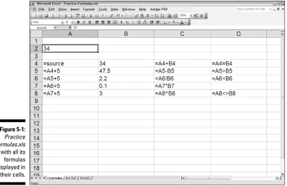
Printing the spreadsheet formulas...46
Chapter 4: Modifying the Spreadsheet ...49
Finding and Opening the Workbook for Editing...49
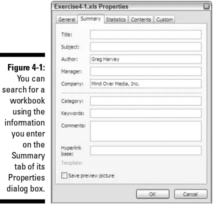
Adding summary information to a workbook ...49
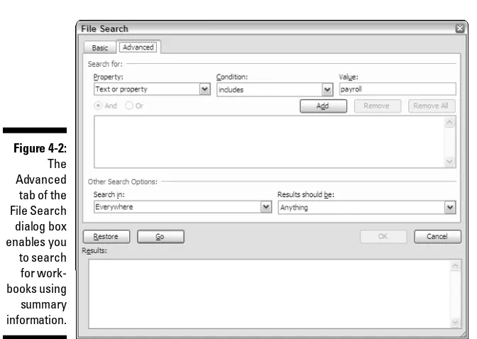
Searching for workbook files ...51
Exploring the Open options ...53
Finding and Identifying the Region that Needs Editing...54
Selecting the Ranges to Edit ...56
Editing Data Entries ...57
Catching Errors with Text to Speech...58
Deleting and Inserting Data and Cells ...60
Moving and Copying Data and Cells ...61
Using Notes in the Spreadsheet ...64
Using Find and Replace and Spell-Checking ...66
Group Editing...68
Part II: Using Formulas and Functions...71
Chapter 5: Building Formulas ...73
Building Formulas ...73
Building formulas by hand ...74
Building formulas with built-in functions...78
Editing formulas ...81
Altering the natural order of operations ...82
Using External Reference Links...84
Controlling When Formulas Are Recalculated ...86
Chapter 6: Copying and Correcting Formulas...89
Copying Formulas with Relative References ...89
Copying Formulas with Absolute References...91
Copying Formulas with Mixed References...92
Using Range Names in Formulas ...96
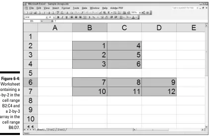
Building Array Formulas ...99
Tracing and Eliminating Formula Errors...101
Dealing with Circular References ...104
Chapter 7: Creating Date and Time Formulas ...107
Constructing Date and Time Formulas ...107
Working with the Date Functions...109
Chapter 8: Financial Formulas and Functions ...115
Working with Financial Functions...115
Using the Basic Investment Functions ...116
Figuring the Depreciation of an Asset ...121
Chapter 9: Using Math Functions...125
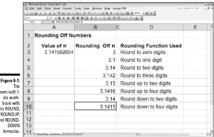
Rounding Off Values...125
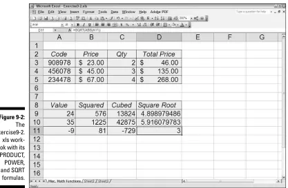
Finding Products, Powers, and Square Roots ...127
Doing Fancier Sums ...129
Summing products, squares, and their differences ...128
Conditional totals ...131
Chapter 10: Using Statistical Functions ...135
Computing Averages...135
Finding the Highest and Lowest Values...136
Counting Cells...137
Using the Statistical Functions in the Analysis ToolPak Add-in...139
Chapter 11: Using the Lookup Functions ...141
Returning Single Values from a Lookup Table ...141
Performing a horizontal lookup ...142
Performing a vertical lookup ...144
Using the Lookup Wizard ...146
Chapter 12: Using the Logical Functions...149
Working with the Logical Functions ...149
Constructing Decision-Making Formulas ...150
Selecting between alternate values...150
Selecting between alternate calculations...153
Nesting IF functions ...155
Constructing Error-Trapping Formulas...157
Chapter 13: Text Formulas and Functions ...161
Constructing Text Formulas ...161
Using Text Functions ...164
Part III: Working with Graphics ...169
Chapter 14: Charting Spreadsheet Data ...171
Understanding Excel Charts ...171
Creating Charts ...176
Formatting Charts ...180
Editing Charts...182
Chapter 15: Adding Graphics to the Spreadsheet...185
Understanding Graphic Objects...185
Using the Drawing Toolbar ...189
Inserting clip art ...189
Importing graphics files...192
Drawing and adding graphic shapes...194
Adding text boxes...196
Part IV: Managing and Securing Data ...201
Chapter 16: Building and Maintaining Data Lists...203
Creating a Data List...203
Sorting Lists ...207
Using sorting keys ...207
Sorting on more than three keys ...209
Sorting the fields (columns) in a data list ...209
Subtotaling a List ...211
Filtering a List ...213
Querying External Database Tables...216
Chapter 17: Protecting the Spreadsheet...221
Password-Protecting the Workbook ...221
Protecting the Worksheet ...224
Doing Data Entry in a Protected Worksheet ...227
Protecting the Entire Workbook...228
Part V: Doing Data Analysis ...231
Chapter 18: Performing What-If Analysis...233
Using Data Tables...233
Creating single-variable data tables...233
Creating two-variable data tables ...236
Exploring Various Scenarios ...238
Performing Goal Seeking ...240
Creating Complex Models with Solver ...241
Chapter 19: Generating Pivot Tables ...245
Understanding Pivot Tables...245
Creating Pivot Tables...247
Modifying the Pivot Table ...250
Modifying the table formatting...250
Pivoting the table’s fields ...251
Changing the table summary function and adding calculated fields ...252
Creating Pivot Charts ...254
Part VI: Excel and the Web ...259
Chapter 20: Publishing Spreadsheets as Web Pages ...261
Saving Worksheets as Web Pages ...261
Creating static Web pages ...262
Creating interactive Web pages...263
Web pages with interactive data tables...264
Web pages with interactive data lists ...266
Web pages with interactive pivot tables ...267
Web pages with interactive charts...268
Exporting an interactive Web page to Excel ...269
Chapter 21: Adding Hyperlinks to Spreadsheets ...273
Creating Hyperlinks ...273
Adding links to other sheets in a workbook ...274
Adding links to other documents...275
Adding links to Web pages ...277
Editing Hyperlinks...279
Assigning Links to Toolbars and Menus ...279
Part VII: Macros and Visual Basic for Applications...283
Chapter 22: Using Macros...285
Creating Macros ...285
Using the macro recorder ...285
Recording macros with relative cell references ...288
Assigning Macros to Toolbars and Menus...290
Chapter 23: Using the Visual Basic Editor ...293
Using the Visual Basic Editor ...293
Editing a recorded macro...295
Adding a dialog box that processes user input...297
Creating User-Defined Functions ...300
Using a custom function in your spreadsheet...302
Saving custom functions in add-in files ...303
Part VIII: The Part of Tens ...307
Chapter 24: Top Ten Tips for Using Excel like a Pro...309
Generate New Workbooks from Templates ...309
Organize Spreadsheet Data on Different Worksheets...310
Create Data Series with AutoFill...310
Use Range Names...311
Freeze Column and Row Headings...312
Prevent Data Entry Errors with Data Validation ...312
Trap Error Values in Their Original Formulas ...313
Save Memory by Using Array Formulas...313
Controlling the Display of Data in Tables through Outlines...314
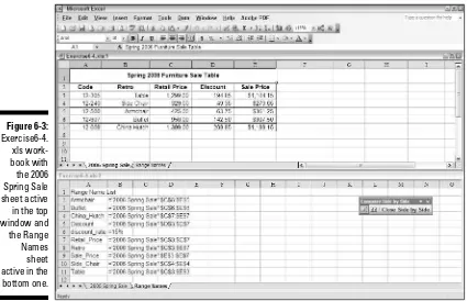
Use Compare Side by Side to Work with Two Workbooks...314
Chapter 25: Ten (More or Less) Shortcut Keys for Entering Data...317
Chapter 26: Ten (More or Less) Shortcut Keys for Formatting the Worksheet ...319
Chapter 27: Ten (More or Less) Shortcut Keys for Editing Data ...321
Chapter 28: Ten (More or Less) Miscellaneous Shortcut Keys ...323
Appendix A: About the CD ...325
Appendix B: Table of Exercises ...329
E
xcel is the most sophisticated spreadsheet program available in the world of personal computing. As such, this program is much more than just an electronic version of an accountant’s familiar green sheet for crunching numbers. For millions of users the world over, Excel is also their number one forms designer, their interface to the corporate data-base, as well as their premier charting program.Given Excel’s indisputable versatility, it should come as no surprise that mastering the basics of the program, not to mention its finer points, is no small undertaking. My experience, how-ever, in teaching adults to use all manner of Excel’s capabilities has convinced me that this mastery is greatly accelerated with just a modicum of hands-on experience judiciously applied to rather simple butrealistic data-related problems.
About This Book
As its name suggests, Excel Workbook For Dummiesis designed to give you the kind of hands-on experience with all the major aspects of the program you need to start using the program for business or home with a certain degree of confidence and efficiency. As you’d expect from this type of book, the workbook is primarily composed of questions and exercises that give you plenty of opportunities to experience the purpose and benefits of Excel’s many features.
It’s my hope that as a result of doing the exercises in this workbook, you’ll not only be in firm command of the basic skills necessary to work with confidence in the Excel spreadsheet but also have a good idea of the overall power of the program through experience with its fea-tures beyond the spreadsheet.
Conventions Used in This Book
By convention, all the text entries that you type yourself appear in bold. In addition, all file-names appear in italicized type even though they are not italicized when you see their file-names in Windows Explorer or the Excel Open dialog box.
When it comes to instructions in the exercises throughout the workbook, you’ll notice two conventions:
⻬Menu commands are introduced by the word “choose” followed by the menu sequence separated by the ➪symbol, as in “Choose File➪Save As.”
⻬Selections in dialog boxes are most often introduced by the word “select” followed by the name of the option name or button, as in “Select the Alignment tab” or “Select the OK button.”
Alt key and then pressing the menu’s and menu items’ hot keys. In the case of dialog box options, you have a choice between clicking them with the mouse or pressing their hot keys. You can also select default buttons in a dialog box (indicated by shading around the button) by simply pressing the Enter key.
The method you use for selecting commands and dialog box options is completely up to you and should be dictated by your comfort level with the mouse or keyboard as well as which method is most efficient. For example, pressing the Enter key to select the default OK button in a dialog box is often the most efficient method when the next step you take is entering or editing in the current cell or range.
One other convention that you’ll notice used throughout the text is the display of the names for Excel menu commands, toolbar buttons, and dialog box options in the title case, wherein all major words are capitalized except for prepositions. The title case is used to make these names stand out from the rest of the text. Often, however, espe-cially in the case of dialog box options, Microsoft does not always follow this conven-tion, often preferring to capitalize the first letter of the option name.
Foolish Assumptions
I assume that you’re a new Excel user motivated to master its essentials either for work or at home. Further, I assume that you’re someone who learns by doing as least as well, if not better than, by reading alone.
To complete most of the exercises in this workbook, you only need to have Microsoft Excel installed on a computer running a version of Microsoft Windows. For some of the printing exercises, you will benefit from having a printer installed on your system (although you can complete most of their steps and get the gist of the lesson without actually printing the sample worksheets). For a few of the Web exercises in Part VI, you
willneed to have access to the Internet in order to complete them.
The workbook is designed to be used with various versions of Excel; from Excel 2000 up to and including Excel 2003. There are, however, a few exercises that are designed pri-marily for users of Excel 2003, whose specific steps require slight modification in order to be accomplished on earlier versions. Only in the rarest of cases will you encounter an exercise that cannot be completed with all three versions. If you are a user of Excel 97, you can complete the majority of the exercises in the workbook, although you may find some of the steps confusing as they reference toolbar buttons or task pane com-mands that haven’t yet been invented as far as your edition of Excel is concerned.
How This Book Is Organized
Part I: Creating Spreadsheets
This part contains the most exercises of any in the workbook. It is made up of four chapters designed to give you practice in all the spreadsheet basics, all the way from starting Excel to editing a completed spreadsheet:
⻬Chapter 1 enables you to practice creating a new spreadsheet.
⻬Chapter 2 runs you through formatting spreadsheet data.
⻬Chapter 3 gives you training in all aspects of printing the completed spreadsheet.
⻬Chapter 4 gives you plenty of experience with making modifications to the com-pleted spreadsheet.
Part II: Using Formulas and Functions
This part gives you all the practice you need with creating and using formulas in the spreadsheet. Chapter 5 introduces you to formula-making just as Chapter 6 introduces you to the all-important topic of formula copying.
Because of the importance of Excel’s built-in functions in formula building, the remaining seven chapters in this part concentrate on building formulas using a particular category of functions:
⻬Chapter 7 gets you up and running on date and time formulas.
⻬Chapter 8 trains you in the use of financial formulas.
⻬Chapter 9 gives you practice creating formulas using Excel’s Math functions.
⻬Chapter 10 concentrates on exercises in creating formulas using Statistical functions.
⻬Chapter 11 introduces you to the creation of formulas using Lookup functions.
⻬Chapter 12 runs you through the creation of formulas using the Logical func-tions, the performance of which depends upon prevailing conditions in the spreadsheet.
⻬Chapter 13 introduces you to the creation of text formulas that manipulate and change text entries in the spreadsheet.
Part III: Working with Graphics
This part takes you into the graphical aspects of Excel, the most important of which is its rich and versatile charting capabilities covered in Chapter 14. In addition to charts, in Chapter 15 you get practice in working with other types of graphics in the spread-sheet, both those that you generate with the program’s own drawing tools and those that you import from other sources such as clip art and digital photos.
Part IV: Managing and Securing Data
maintaining, sorting, and querying database tables and data lists in the worksheet. Chapter 17, on the other hand, gives you practice using Excel’s various methods for protecting your data and worksheets from illicit viewing and unwanted changes.
Part V: Doing Data Analysis
This part takes you to the next step of using the Excel spreadsheet by introducing you to two different kinds of data analysis. Chapter 18 gives you practice in doing various types of what-if analysis that enable you to look at different potential outcomes in the spreadsheet. Chapter 19 concentrates on training you in the use of pivot tables, a dynamic type of data table that you can use to summarize vast amounts of data.
Part VI: Excel and the Web
This part gives you experience with Excel’s Web capabilities in two forms. Chapter 20 gives you experience converting Excel spreadsheets to Web pages, both in static and dynamic formats. Chapter 21 trains you in the use of hyperlinks in spreadsheets that connect you to different sheets in the same workbook, different documents on the same computer, as well as to different pages and e-mail addresses on the World Wide Web.
Part VII: Macros and Visual Basic
for Applications
This part introduces you to the topic of creating and using macros to both streamline and customize your work in Excel. Chapter 22 introduces you to recording your actions as Excel macros and then playing them back in the worksheet. Chapter 23 gives you practice using Excel’s Visual Basic Editor to edit macros and extend macros you’ve recorded as well as to create your own user-defined functions.
Part VIII: The Part of Tens
This part gives you tips for using Excel on your own after you complete the exercises in this workbook. Chapter 24 is full of tips on using some of the many features you’ve practiced using in the workbook like a professional. Chapters 25 through 28 are full of various and sundry keystroke shortcuts designed to save you keyboard enthusiasts out there all sorts of time as you work in Excel.
Using the Practice Material on the CD-ROM
The CD-ROM that comes with this workbook is an integral part of the workbook experi-ence. It contains not only the practice material that you need to complete most of its exercises but lots of third-party utilities that you may be able to put to good use as you start to work with Excel on your own.
Before you start working through the exercises in this workbook, I suggest that you copy this Excel Workbook folder to the My Documents folder on your computer’s hard disk and then rename the Excel Workbook folder to My Practice Spreadsheets as follows:
1.
Insert the CD-ROM into your computer’s CD/DVD drive.2.
Click the Start button on the Windows taskbar and then click My Computer on the Start menu to open My Computer in Windows Explorer.3.
Right-click the icon for your CD/DVD drive and select Explore to open its con-tents in the Windows Explorer window.4.
Click the Excel Workbook folder icon and then press Ctrl+C.5.
Click the My Documents link in the left pane of the Windows Explorer window and then press Ctrl+V.6.
Right-click the Excel Workbook folder and then select the Rename option on its shortcut menu.7.
Replace Excel Workbook by typing My Practice Spreadsheetsand then press Enter.8.
Click the Close button in the upper-right corner of the Windows Explorer window to close it.9.
Open the My Practice Spreadsheets folder in My Documents on your hard disk and then open the Templates folder. Select all the files by pressing Ctrl+A and copy them to the Windows Clipboard by pressing Ctrl+C.10.
Open the Microsoft Templates file on your computer’s hard disk by double-click-ing the My Computer icon on the desktop and then double-clickdouble-click-ing the Local Disk (C:) icon followed by the following folders: Document and Settings➪Your personal folder (as in Greg) ➪Application Data➪Microsoft➪Templates.If the Application Data folder icon does not appear in your personal folder, you need to choose Tools➪Folder Options and then select the Show Hidden Files and Folders option button on the View tab before you select OK.
11.
Paste the copied template files into the Templates folder by pressing Ctrl+V.You are now ready to tackle any of the exercises in the workbook using the practice files saved in the My Practice Spreadsheets folder inside the My Documents folder on your hard disk.
When you’re finished doing the exercises and no longer need access to the practice files, go ahead and delete the My Practice Spreadsheets folder and all its contents by dropping it in the Recycle bin on the Windows desktop.
Icons Used in This Book
Icons are sprinkled throughout the text of this workbook in high hopes that they draw your attention to particular features. Some of the icons are of the heads-up type, while others are more informational in nature:
This icon indicates the start of a question-and-answer section in the workbook.
This icon indicates a hint that can help you perform a particular step in the exercise.
This icon indicates that the file referred to in an exercise or some part of it is supplied to you on the CD-ROM that comes with this workbook.
This icon indicates a tidbit that, if retained, can make your work somewhat easier in Excel.
This icon indicates a tidbit that is essential to the topic being discussed and is, there-fore, worth putting under your hat.
This icon indicates a bit of trickery in the topic that, if ignored, can lead to some real trouble in your spreadsheet.
Where to Go from Here
This workbook is constructed such that you don’t have to start working through the exercises in Chapter 1 and end with those in Chapter 23. That being said, it is still to your benefit to complete all the exercises within a particular chapter, if not in a single work session, at least in a short time period.
If you’re a real newbie to Excel and have no experience with the program, I urge you to complete the exercises in Part I, Chapters 1 through 4, before you take off in your own direction. The exercises in this part are truly fundamental and are meant to give you a strong foundation in the basic features that all Excel users need to know.
Please keep in mind that I designed the exercises in this workbook to work with my Excel companion books,Excel For Dummiesand Excel All-In-One Desk Reference For Dummies (published by Wiley). They can therefore provide you with additional infor-mation about the Excel features you’re using either at the time you go through the workbook exercises or afterward. To facilitate this crossover usage, I have, wherever possible, used the same example files in the exercises of this workbook as you see illustrated and explained at length in these references.
Entering the
Spreadsheet Data
In This Chapter
䊳Launching Excel and opening a new workbook
䊳Moving around the workbook
䊳Selecting cell ranges in a worksheet
䊳Doing simple data entry in a worksheet
䊳Using AutoFill to create data series and copy formulas
䊳Saving the spreadsheet as an Excel workbook file
D
ata entry is the bread and butter of any spreadsheet you create or edit. The exercises in this chapter give you a chance to practice launching Excel, moving around a new spreadsheet, the many aspects of data entry, and, most importantly, saving your work.Launching Excel
Excel is only one of the many application programs included as part of Microsoft Office. In order to be proficient in its use, you need to be familiar with all the various ways of launch-ing the program.
Q.
What are the different techniques I can use to start Excel?A.
You should be familiar with all these methods:• Click Start on the Windows taskbar and then highlight All Programs and click Microsoft Office Excel (2003 users need to select the Microsoft Office item before clicking Microsoft Office Excel).
• Double-click an Excel workbook file in any folder on any drive to which your computer has access.
• Double-click the Excel program icon on your computer’s desktop.
• Click the Microsoft Excel icon on the taskbar’s Start menu.
Exercise 1-1: Launching Excel
The last three methods listed previously for launching Excel are available only if you’ve added the Excel program icon to the desktop, the Start menu, and the Quick Launch toolbar, respectively. For this exercise, add the Excel program icon to your computer if you still need to and then launch Excel using each of the five methods.
⻬Add an Microsoft Office Excel shortcut to the Windows desktop by right-clicking the Microsoft Office Excel item as it appears on the Start➪All Programs➪ Microsoft Office submenu and then highlighting Send To before you click Desktop (Create Shortcut) on the Send To submenu.
⻬Add Excel to the Start menu by right-clicking the Microsoft Office Excel desktop shortcut and then clicking Pin to Start Menu on its shortcut menu.
⻬Add Excel to the Quick Launch toolbar on the Windows taskbar by holding down Ctrl as you drag and drop the Microsoft Office Excel desktop shortcut on to its place in the toolbar.
Try It
Q.
How do I make Excel launch automatically each time I start my computer?A.
Copy the Microsoft Office Excel item to the Startup submenu on the All Programs menu.Opening a New Workbook
Each time you launch Excel (using any method other than double-clicking an Excel file icon), a new workbook containing three blank worksheets opens. You can then build your new spreadsheet in this workbook, using any of its sheet pages.
The blank workbook that opens with Excel is given a temporary filename such as Book1, Book2, and so on that appears after Excel’s name on the program window’s title bar. If you want to start work on a spreadsheet in another workbook, click the New button on the Standard toolbar.
When Excel opens a blank workbook upon launching the program or after clicking the New button, the new workbook follows the general Excel Worksheet template (which controls the formatting applied to all its blank cells). You can also open new workbooks from other, specialized templates or from a workbook that you’ve already created. To do this, choose File➪New. If you’re running Excel 2002 or 2003, the program opens the New Workbook Task pane, where you can click the template or file to use. If you’re running Excel 2000 or earlier, the program opens the New dialog box, from which you can open the template.
Exercise 1-2: Opening a New Workbook
Launch Excel and then open a new workbook (Book2). Switch to Book1 (notice the change in the Excel program title bar) and then back to Book2 and close this work-book. Notice what happens to Book1 when you close Book2. Leave Book1 open for the next exercise.
To switch from Sheet1 of Book2 and make Sheet1 of Book1 active, click the Book1 icon on the Windows taskbar or press Ctrl+Tab (to switch back to Book2, click the Book2 icon on the taskbar or press Ctrl+Tab again so that Sheet1 of Book2 is selected).
To close a workbook file, choose File➪Close or click the workbook’s Close Window button. (The Close Window button is the one with the black X, which is immediately beneath the program’s red Close button, which has a white X.)
Exercise 1-3: Opening a New Workbook from a Template
Open a new workbook from the Hourly Wages template that you copied from the Templates folder on the workbook CD-ROM to the Microsoft Templates folder (see “Using the Practice Material on the CD-ROM” in the Introduction for details). Switch back and forth between the Book1 and Hourly Wages1 workbook files. Then, close the Hourly Wages1.xls workbook file, leaving open the Book1.xls file for the next exercise.
To open a new workbook from a template file, you click the On My Computer link under Templates on the New Workbook task pane, and then click the .xlt file to use in the General tab of the Templates folder before you select OK.
Try It
Q.
What’s so special about an Excel template?A.
A template is a particular type of Excel filedesigned to automatically generate new workbooks that use both its data and for-matting. Each time you open a template, Excel opens a copy of the template file rather than the original (by appending a number to the template’s original name). Excel template files use the file-name extension .xlt to differentiate them from regular Excel workbook files, which carry an .xls filename extension.
Q.
What’s the difference between opening a new workbook file from an Excel template file rather than an existing Excel workbook file?A.
None, provided that you open the new file using the From Existing Workbook under New or the On My Computer link under Templates in the New Workbook Task pane, rather than in the Open dialog box. (Doing this opens not a copy of the template or workbook file but the original file for editing.)Q.
How can I create templates out of my own Excel workbook files?A.
Build a spreadsheet in a new or existing workbook file. To this spreadsheet add all the stock text and data, calculating formu-las, and formatting required in all the filesMoving around the Workbook
The key to doing both data entry and data editing in any spreadsheet is selecting the cell or cells you want to fill or modify. Selecting a cell almost always entails moving the cell cursor (or pointer) to another part of the current worksheet. Sometimes, it also involves activating a different worksheet in the workbook file.
Excel gives you plenty of choices in techniques for moving the cell cursor: Some use the mouse and others are keyboard driven.
Moving within the displayed area
Here’s a recap of the most important ways to move the cell cursor to a new cell within the area of the worksheet that is currently displayed on-screen:
⻬Click the target cell with the white-cross mouse pointer.
⻬Press the arrow keys until the cell pointer is in the target cell.
⻬Click the Name Box with the current cell reference at the very beginning of the Formula Bar, enter the reference of the target (by column letter and row number as in D12), and press Enter.
Exercise 1-4: Moving the Cell Cursor within the Displayed Area
Make Sheet1 of the blank workbook, Book1, active and then practice moving the cell cursor to different cells in the displayed area using the mouse, arrow keys, and Name Box:
1.
Move the cell pointer to cell F9 with the mouse.2.
Move the cell pointer to cell C13 using just the down and left arrow keys.3.
Move the cell pointer to cell A1 using only the Name Box.Keep in mind that you can always move the cursor to cell A1 (also known as the Home cell) of any active worksheet simply by pressing Ctrl+Home.
Moving to a new area of the worksheet
Many times you have to make cell entries in areas that aren’t currently displayed in the active worksheet. One of quickest ways to do this is by entering the reference of the cell you want to go to in the Name Box. You can also use any the following techniques to scroll to new parts of the current worksheet:
⻬To scroll up and down rows of the worksheet by windows, press Page Up or Page Down or click the blank area above or below the scroll box in the vertical scroll bar.
⻬To scroll left and right columns of the worksheet by windows, click the blank area to the left or right of the scroll box in the horizontal scroll bar.
⻬To quickly scroll through rows or columns of the worksheet, hold down the Shift key as you drag the scroll box up or down in the vertical scroll bar or left and right in the horizontal scroll bar.
⻬If you use a mouse with a wheel button, scroll up and down the rows of the work-sheet by rotating the wheel button forward (to scroll up) and backward (to scroll down).
⻬If you use a mouse with a wheel button, pan through the rows and columns of the worksheet by clicking the wheel button and then dragging the triangular mouse pointer in the direction you want to scroll.
Don’t forget that scrolling is not the same as selecting! After scrolling to a new part of the worksheet in view, you still have to select a cell by clicking it to set the cursor in it.
Exercise 1-5: Moving the Cell Cursor to Distant Parts of the Worksheet
Practice moving the cell pointer to cells in unseen parts of Sheet1 in the Book1 work-book by doing the following:1.
Move the cell cursor to cell C125 with the Name Box on the Formula Bar.2.
Move the cell cursor to cell CA125 using the horizontal scroll bar.3.
Move the cell cursor to cell CA63560 using the vertical scroll bar.4.
Move the cell cursor directly to cell A1 (the Home cell) in a single operation. Hold down the Shift key to scroll quickly through columns and rows by dragging the scroll box in the horizontal or vertical scroll bar.After scrolling into view the region with the cell you want to select, you still need to click the cell to select it.
Try It
Q.
What’s the most efficient way to move between ranges of data that are spread out across a worksheet?A.
Use the Ctrl key in combination with any of the four arrow keys to jump from occupied cell to occupied cell in a particular direction.Exercise 1-6: Moving the Cell Cursor from Entry to Entry
Practice moving the cell pointer around a blank worksheet and between data entries with the Ctrl key and the arrow keys in Sheet1 of Book1 by doing the following:
1.
Press Ctrl+→, Ctrl+↓, Ctrl+←, and Ctrl+↑in succession to jump the cell cursorfrom A1 to IV1, IV1 to IV65536, IV65536 to A65536, and A65536 to back to A1 (when there are no occupied cells in a particular direction, the cursor jumps right to the border of the worksheet).
2.
Move the cell cursor to cell A18, type Stop, and press Ctrl+Home. Next, press Ctrl+↓(the cursor stops in A18 rather than A65536 because A18 is now occupied).3.
Move the cell cursor to cell AB18, type Stop Again, and press Home. Next, press Ctrl+→(the cursor stops in cell AB18 rather than IV18 because AB18 is nowoccupied).
4.
Press the Delete key, and then press Ctrl+←followed by the Delete key to removethe two dummy cell entries. Press Ctrl+Home to put the cursor back in cell A1.
Moving to a different sheet in the workbook
Each new workbook you start uses the general Excel Worksheet template that auto-matically includes three blank worksheets that you can fill with data. If you need more space for a particular spreadsheet, you can add additional worksheets with the Insert➪Worksheet command. If you want all new workbooks you open to have more worksheets, enter a new value in Sheets in a New Workbook text box on the General tab of the Options dialog box (Tools➪Options).
Each sheet in a workbook is automatically given the next available numeric name such as Sheet1, Sheet2, and the like, but you can easily replace these generic names with something descriptive: Double-click the tab you want to rename, type the new sheet name, and press Enter. You can also color-code a sheet tab by right-clicking it, clicking Tab Color on the shortcut menu, and then selecting the color Format Tab Color dialog box before you select OK.
Of course, you must know how to move between the sheets in order to be able to add and edit data in them. The most direct way to select a new worksheet is to click its sheet tab, although you can also use the shortcut keys Ctrl+Page Down to select the next sheet and Ctrl+Page Up to select the previous sheet.
If you add so many worksheets to your workbook that all their sheet tabs can’t all be displayed at one time, you can use the Tab scroll buttons to the immediate left of the sheet tab to bring into view the tabs you want to select. You can also display more tabs by reducing the width of the horizontal bar (by dragging to the right the split bar that appears when you position the mouse pointer on the vertical bar at the beginning of the scroll bar).
Exercise 1-7: Moving to Different Worksheets
Practice moving the cell cursor to specific cells in different worksheets of Book1 by doing the following:
1.
Move the cell cursor to cell J25 on Sheet2 (whose cell reference is Sheet2!J25).2.
Move the cell cursor to cell CC1000 on Sheet3 (Sheet3!CC1000).3.
Move the cell cursor to cell Sheet 3:J25 on Sheet3, and then activate Sheet2 (note the difference in the worksheet view despite the fact that you’ve moved to the same cell on an earlier worksheet).4.
Rename Sheet1 to Spring Sale.Selecting Cell Ranges
When entering, editing, or formatting a single cell, all you have to do is move the cell cursor to it as you practiced in the earlier exercises. You can also enter the same data as well do the same type of editing and formatting in a bunch of cells at one time, but to do so, you must first select the cells where all this is going to happen.
Most of the time when selecting multiple cells in a worksheet, you select a discrete block of cells of so many rows high and so many columns wide. Such a block is known as a cell rangein the parlance of spreadsheet software.
A cell range is most often described by the reference of its first and last cell (that is, the cell in the upper-left corner and the lower-right corner of is block, respectively). When written, a cell range is separated by a colon, as in B15:F20, for a row and six-column cell range whose first cell is B15 and last cell F20. To select this cell range, you move the cursor to cell B15 and then hold down the Shift key as you use the ↓and →
keys to move the cursor to cell F20.
Excel, however, does not limit you to selecting a single cell range for data entry, edit-ing, or formatting. You can select as many cell ranges (even those as small as a single cell) by holding down the Ctrl key as you add a new range to the cell selection.
Always think of the Shift key when you want to select a single range of cells and the Ctrl key when you want to select more than one cell range at one time.
Q.
How do I select cell ranges that include complete rows and columns of the active worksheet?A.
Click the letter of the column or the number of the row whose cells are to be selected in the column and row header, respectively. To select multiple columns orrows, hold down the Shift key as you drag through them, if they are consecutive, or click them as you hold down the Ctrl key, if they are noncontiguous. Press Ctrl+A or click the box at the junction of the column and row header to select all the columns and rows in the active worksheet (in other words, the entire worksheet).
Exercise 1-8: Selecting Various Cell Ranges
Practice selecting cell ranges in the Spring Sale worksheet of Book1 by doing the following:
1.
Select the cell range A2:E2, and then click the Fill Color drop-down button on the Formatting toolbar. Click the Gray-25% square in the pop-up color palette.2.
Select the cell ranges A3:A9 and B3:E3 as a single cell selection (I’m sure you canConTRoL it) and then assign Light Turquoise to it using the Fill Color drop-down button.
3.
Select the cell range B4:E9 and then assign Light Yellow to this range using the Fill Color drop-down button. Next, move the cell cursor to cell A1 (Home).Making Cell Entries
As you are probably already aware, Excel recognizes only two types of cell entries, text (label) and number (or value). Numeric cell entries are those that consist solely of
Try It
Q.
How do I select cell ranges that span differ-ent worksheets of the active workbook?numbers or calculable formulas. Text entries are those that consist of all letters or a combination of letters, numbers, and punctuation on which Excel can perform no sort of calculation.
Anything you enter into a cell or cell selection is immediately analyzed as either being a number or text entry. Because the general Excel Worksheet template automatically left-aligns all text entries and right-aligns all numeric ones, you can often tell immedi-ately how your entry has been classified by noting how it’s aligned in its cell.
When you make a numeric entry in a worksheet, Excel not only right-aligns the value in its cell but also assigns the General number format to it. In this format, only significant digits are displayed. This means that all trailing zeros are dropped. Also, if the number you enter contains more that can fit within the current column width, Excel automati-cally converts the value to scientific notation (as in 5.00E+09 for 5,000,000,000).
Sometimes you have to override Excel’s number/text assignment in order to obtain the desired cell entry. The most famous example of this is a ZIP code or all numeric part or item number that begins with a zero, as in 00105. If you try to enter this ZIP code into a cell simply by typing its five digits, Excel will interpret it as a numeric entry and in assigning the General format to it, retain only the value 105 in the cell. In order to retain the preceding zeros, you need to force the entry to be recognized as text by typing an initial apostrophe as in '00105(this apostrophe does not appear in the cell although you can see it on the Formula bar).
Entering data in a single cell
Most cell entries are made by typing from the keyboard (although later versions of Excel do support voice and ink text entry). After typing the characters, which appear both in the cell and on the Formula bar, you must still complete the entry.
Anytime prior to completing the cell entry, you can press the Esc key to clear the cell of all characters you typed there.
Q.
How many methods can I use to complete an entry in the current cell?A.
You should be familiar with all these methods:• Click the Enter box on the Formula bar (the one with the check mark).
• Press the Enter key.
• Press one of the arrow keys.
• Press Tab, Shift+Tab, Home, Ctrl+Home, Page Up, Page Down, Ctrl+Page Up, Ctrl+Page Down, or any of the other cursor-movement key combinations
Exercise 1-9: Making Simple Data Entries
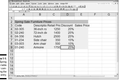
Complete the data entry for the simple Spring Sale table shown in Figure 1-1 by doing the following:
1.
Enter the table title Spring Sale Furniture Pricesin cell A2.2.
Enter the column headings in row 3 as follows:•Codein cell A3
•Descriptionin cell B3
•Retail Pricein cell C3
•Discountin cell D3
•Sales Pricein cell E3
3.
Enter the code numbers in column A as follows: •02-305in cell A4•02-240in cell A5
•04-356in cell A6
•01-234in cell A7
•03-003in cell A8
•01-240in cell A9
4.
Enter the furniture descriptions in column B as follows: •36-inch round tablein cell B4•72-inch dining tablein cell B5
•Hutchin cell B6
•Side chairin cell B7
•Arm chairin cell B8
•Armoirein cell B9
5.
Enter the retail prices of the furniture in column C as follows: •1250in cell C4•1400in cell C5
•2500in cell C6
•350in cell C7
•500in cell C8
•1750in cell C9
6.
Enter the discount percentages in column D as follows: •25%in cells D4, D5, and D6•15%in cells D7 and D8
•25%in cell D9
Check your completed spreadsheet table against the one in Solved1-9.xls.(Open this workbook in the Chap1 folder inside the My Practice Spreadsheets folder that you’ve created in your My Documents folder your hard disk, or in the Excel Workbook folder on the CD-ROM that came with this book.)
Entering data in a cell range
Sometimes you want to make the same entry in several different cells in the same worksheet. To do this, select all the cells and cell ranges and then press Ctrl+Enter to both complete the entry you make in the active cell and simultaneously insert it into all the other selected cells.
Filling in a data series with the Fill handle
The tiny black square in the lower-right corner of the cell cursor is known as the Fill handle. The Fill handle is your key to the AutoFill feature that makes it super-easy either to fill in a continuous range with the same entry or with data series (such as Monday, Tuesday, Wednesday, and so on, or 101, 102, 103, and the like).
To create a sequential series that increments by one unit (day, hour, month, widget number), you enter the first entry in the series in a blank cell and then drag the Fill handle in the direction you want the series to appear (down or to the right are the most common directions). To create series that increments by other units (every other day, every third month, every fourth hour, every tenth widget), you enter the first two entries in the series (that serve as an example of the increment to be used) in two adjacent blank cells and then drag the Fill handle in the appropriate direction.
Figure 1-1:
Instead of filling in these recognized data series with AutoFill, you can force Excel to copy the entry you’ve made in the current cell by holding down the Ctrl key as you drag the Fill handle. Excel indicates that it copied rather than filled a range by display-ing a tiny plus sign to the side of the Fill handle mouse pointer.
Exercise 1-10: Entering the Same Entry and Using AutoFill
Open a new blank workbook, Book2, and then practice making the same data entry in multiple ranges and using the Fill handle to create various data series in its Sheet1:
1.
Enter today’s date, following the date format Oct-25-06, in the cell selection A1, D3:F3, and B4:B6.• Don’t forget to hold down the Ctrl key when you’re selecting the three ranges in the cell selection.
• Be sure to complete the current date entry into all the cells of the selection by pressing Ctrl+Enter.
2.
Use AutoFill to create a data series with all 12 months in the cell range A8:A19 starting with January.3.
Use AutoFill to create a data series with the names of all the days of the week in cell range C8:I8 starting with Monday.4.
Use AutoFill to create a data series with hours that go from 8:00AMto 8:00PM in cell range C10:C22.5.
Use AutoFill to create a data series in cell range E10:H10 containing the headings Qtr1, Qtr2, Qtr3, and Qtr4.6.
Use AutoFill to create a series in cell range E12:E21 containing 1st Team, 2nd Team, 3rd Team, and so on all the way up to 10th Team.7.
Use AutoFill to create a data series in cell range G12:L12 that contains the name of every other month starting with Novemberand ending with September.• Don’t forget that you need to indicate the every-other-month increment to Excel (by entering January in cell H12 and then selecting the range G12:H12) before using the Fill handle to create the data series.
8.
Use AutoFill to copy the data entry Item 1to the entire cell range G14:G19 (don’t let this one get out of ConTRoL).Copying a formula with the Fill handle
AutoFill is not only useful for filling in a data series or copying a static data entry to a continuous cell range but also for copying a formula across a row or down a column of a data table. When you copy a formula, Excel automatically adjusts the column and row references in the copies so that they refer to the right data.
Don’t forget that Excel automatically uses the so-called relative column and row refer-ences cell addresses in all formulas you create. If you ever need to override this so that all or part of a cell reference is not adjusted in the copied formulas, you enter a $ (dollar sign) before the cell’s column letter or row number (you can have Excel do it for you by pressing F4 while building the formula on the Formula bar).
Exercise 1-11: Copying a Formula with AutoFill
Complete the Spring Sale table by using the following steps to enter the formula that calculates the sales price in cell E4 and then use AutoFill to copy that formula down the cell range E5:E9. (Check your results against those in the Spring Sale table shown in Solved1-11.xls. You can find this workbook in the Chapter 1 folder in the My Practice Spreadsheets folder in the My Documents folder on your hard disk or in the Excel Workbook folder on the CD-ROM that comes with this book.)
1.
Switch to the Spring Sale sheet of Book1 and then move the cell cursor to cell E4.2.
Type =(equal) to start the formula for calculating the sale price of the 36-inchround table (all Excel formulas start with the equal sign).
3.
Click cell C4, and then type *(asterisk), which Excel uses as the sign of multiplica-tion, before you click cell D4 (the formula now reads =C4*D4 on the Formula bar).4.
Click the Enter box on the Formula bar and then drag the Fill handle of the cellcursor in cell E4 down to E9 and release the mouse button to make the copies of the formula.
Saving the Spreadsheet in a Workbook File
Now all that remains to do is to save the spreadsheets you created while performing the exercises in this chapter before exiting Excel. As you know, all work that you do in between the times you save the worksheet is at risk because you immediately lose it if your computer experiences even the briefest power interruption.
The first time you save your spreadsheet in a workbook file, the Save As dialog box appears, giving you the opportunity to rename the file (replacing the Book1, Book2 monikers with something more descriptive) in the File Name text and indicate the folder in which it should be saved in the Save In drop-down list box. After that, you can use the Save command to save all additional changes to the same file without opening any dialog box.
Excel saves the current position of the cell cursor in the worksheet when you save its workbook. Therefore, always position the cursor in the cell you want to be current when you next open the workbook for editing before doing the final save of your work session.
Try It
Q.
How many different techniques can I use to save changes to my workbook file?A.
You should be familiar with all these methods:• Click the Save button on the Standard toolbar (the one with the disk icon).
• Choose File➪Save on the Menu bar (choose File➪Save As if you want to open the Save As dialog box again so that you can rename or save a copy in a new folder).
Exercise 1-12: Saving a Spreadsheet
Save the Spring Sales table in a new My Spreadsheets folder inside the My Documents folder on your hard disk:
1.
With the Spring Sales table displayed on-screen, select cell A2 before you open the Save As dialog box and then click the New Folder button in the Save As dialog box.2.
Type My Spreadsheets(or My Practice Spreadsheetsif you already have a My Spreadsheets folder inside the My Documents folder) as the folder name in the Name text box of the New Folder dialog box and select OK.3.
Replace Book1.xls in the Name text box by typing Spring Furniture Saleand then clicking the Save button.4.
Close the Spring Furniture Saleworkbook and then switch to Sheet1 of Book2. Save this spreadsheet in the My Spreadsheets folder with the filename AutoFill Practiceafter positioning the cell cursor in cell A1.5.
Close the AutoFill Practiceworkbook and the Hourly Wages1workbook by exiting Excel (File➪Exit or Alt+F4) — don’t save your changes to the Hourly Wages1workbook.
Formatting the
Spreadsheet
In This Chapter
䊳Resizing columns and rows in a worksheet
䊳Formatting cells with the Formatting toolbar
䊳Formatting cells with the Format Cells dialog box
䊳Formatting tables with AutoFormat and ranges with Format Painter
䊳Using Conditional Formatting
䊳Hiding columns and rows in a worksheet
I
n Excel, formatting means formatting cells of the worksheet. Therefore, the formatting you assign a cell not only affects the cell’s current contents, but any contents you enter into it. Performing the exercises in this chapter gives you a chance to practice widening and narrowing the columns of rows of a worksheet to suit the formatting and contents of its cells. You also discover a full array of techniques for assigning formatting to cells in a worksheet, including using the Formatting toolbar and the Format Cells dialog box and the AutoFormat and Conditional Formatting features.Resizing Columns and Rows
In all new workbooks generated from the general Excel Worksheet template, all the columns of its worksheets are a standard 8.43 characters or 64 pixels wide, and all the rows are 12.75 points or 17 pixels high. You can, if you need, change this default column width for an entire worksheet by clicking its sheet tab to select it before choosing Format➪Column➪Standard Width on the Excel menu bar. Then, you enter the new default width in the Standard Column Width text box (in characters) before you select OK.
Making column widths suit the data
Resizing particular columns to suit the data they contain is one of the most common formatting tasks you perform in creating and editing a spreadsheet.
You need to widen a column in a worksheet whenever it contains cells with numerical data having too many digits to be displayed in the current column width (indicated by a string of pound signs (#) in the cells) or text data with characters cut off (because they spilled over into cells in columns to the immediate right that were then truncated by entries made in the adjacent column).
Q.
How many different ways should I know for resizing particular columns in a worksheet?A.
You should be familiar with all the follow-ing methods:• Drag the column’s right border in the column header to the left (to narrow) or right (to widen). To resize several columns at once, drag through their column letters in the header or Ctrl+click them before dragging right border of one of them.
• Double-click the column’s right border in the column header to resize it with AutoFit. To resize several columns at once, drag through their column letters in the header or Ctrl+click them before double-clicking the right border of one of them.
• Select the column or columns to resize and then choose Format➪Column➪ Width. Enter the new width (in charac-ters) in the Column Width dialog box before you select OK.
• Select the cell range or selection whose columns need resizing and then choose Format➪Column➪AutoFit Selection. (Excel widens or narrows the columns in the cell selection to display all the digits and text in the cells in the selection.)
• Select the column or columns to resize to standard column width (of 8.43 characters) and then choose Format➪ Column➪Standard Width and select OK in the Standard Width dialog box.
Exercise 2-1: Modifying Column Widths in a Spreadsheet
Launch Excel and then open the Spring Furniture Sale.xlsworkbook you created in doing the exercises in Chapter 1 and saved in the My Spreadsheets (or My Practice Spreadsheets folder). If you didn’t do these exercises, open the Exercise2-1.xlsfile in the Chapter 2 folder.
⻬If you’re using Excel 2002 or 2003, look for the Spring Furniture Sale.xlson the Open Task pane and, if you find it, click its name to open the file. If you’re using an earlier version, open the File menu and then type the number of Spring Furniture Sale.xlsif it’s listed among the four most recently used files at the bottom of the File menu.
⻬If Spring Furniture Sale.xlsis not listed as one of the four most recently used files, click the Open button on the Standard toolbar. Next click the My Documents button on the left pane and double-click the My Practice Spreadsheets folder to display the Chapter 2 folder (which contains the Exercise 2-1.xlsfile). After dis-playing the file to open, click its icon and then select the Open button.
After you open this workbook file, make the following changes to the widths of the columns on the Spring Sales worksheet:
1.
Use the AutoFit feature to widen Column B containing the furniture descriptions sufficiently so that none of these descriptions are cut off.2.
Drag the right border of Column C to the left until the column is 33 pixels wide and then release the mouse button (note the appearance of ### indicators in all but two cells in the Sale table). Next, use AutoFit to widen Column B so that all the entries in this column are displayed.3.
Use the Column Width dialog box to set column E to a width of 10 characters.4.
Narrow column A to 7.14 characters or 55 pixels wide (use any method thatworks).
5.
If you’ve been modifying your Spring Furniture Sale.xlsfile, click the Save button on the Standard toolbar or press Ctrl+S to save your changes. If you’ve been modifying the Exercise 2-1.xlsfile, choose File➪Save As or press F12 to open the Save As dialog box and then rename Exercise 2-1.xlsto Spring Furniture Sale.xlsin the File Name text box. Make sure that the My Practice Spreadsheets folder inside My Documents is selected as the location in the Save In drop-down list before you select Save.Manipulating the height of certain rows
You don’t find yourself having to resize the rows of a worksheet all that much. Most of the time, Excel does all the work for you by automatically resizing them just right to accommodate any and all formatting changes you make to their cells.
About the only time you might want to increase the height of a row on your own is when you want to increase the space between the contents of one row and the con-tents of the row immediately above without going through the trouble of inserting a blank row as a spacer between them.
Q.
How can I manually modify the height of selected rows in a worksheet?A.
You should be familiar with both of these methods for changing row height:• Drag the lower border of the number of the row to modify in the row header either up (to shorten the row) or down (to heighten the row). To modify multiple rows at one time, select the rows (by dragging through or Ctrl+clicking their
row numbers in the row header) and then drag just the lower border of just one of the selected rows.
• Position the cell cursor in any one of the cells in the row to be modified, and then choose Format➪Row➪Height, and then enter the number of points in the Row Height text box before you select OK. To modify multiple rows at one time, select the rows before opening the Row Height dialog box.
Exercise 2-2: Modifying Row Heights in a Spreadsheet
In the Spring Furniture Sale.xlsworkbook, practice modifying row height by doing the following:
1.
Increase the height of Row 2, which contains the table title, to 26.25 or 35 pixels by dragging the row’s border.Note how the spreadsheet title sinks down when the row height is increased.
2.
Restore the height of Row 2 to its original height with AutoFit.Double-click the lower border of a row in the row header to modify its height using AutoFit or place the cell cursor somewhere in the row and choose Format➪Row➪AutoFit.
Cell Formatting Techniques
Cell formatting can run the gamut from changing the font, color, attribute, and/or align-ment of a cell entry to the color, borders, and protection status of the cell itself. You can accomplish much of the formatting in a typical spreadsheet with the buttons on the Formatting toolbar. The rest you can accomplish with the options available on the various tabs of the all-important Format Cells dialog box.
The first rule of formatting is to remember to select all the cells that need formatting before you select the desired button on the Formatting toolbar or an option on one of the tabs in the Format Cells dialog box.
Formatting cells with the Formatting toolbar
The Formatting toolbar shown in Figure 2-1 contains the tools you most often need when formatting your average spreadsheet. These tools are arranged into six groups of buttons (from left to right across the toolbar):
⻬Font and Font Size drop-down buttons
⻬Bold, Italic, and Underline attribute buttons
⻬Left, Right, Center, and Merge and Center alignment buttons
⻬Currency, Percent, and Comma Style buttons along with Increase Decimal and Decrease Decimal buttons
⻬Decrease Indent and Increase Indent buttons
⻬Borders, Fill Color, and Font Color buttons