© 2008 Prentice-Hall, Inc.
Chapter 6
To accompany
Quantitative Analysis for Management, Tenth Edition, by Render, Stair, and Hanna
Power Point slides created by Jeff Heyl
Inventory Control Models
© 2009 Prentice-Hall, Inc. 6 – 2
Introduction
Inventory is an expensive and important
asset to many companies
Lower inventory levels can reduce costs
Low inventory levels may result in stockouts
and dissatisfied customers
Most companies try to balance high and low
inventory levels with cost minimization as a goal
Inventory is any stored resource used to
satisfy a current or future need
Common examples are raw materials,
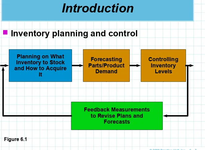
Introduction
Basic components of inventory
planning
Planning
what inventory is to be
stocked and how it is to be acquired
(purchased or manufactured)
This information is used in
forecasting
demand for the inventory
and in
controlling
inventory levels
Feedback
provides a means
to revise
the plan and forecast based on
© 2009 Prentice-Hall, Inc. 6 – 4
Introduction
Inventory may account for 50% of the total
Introduction
All organizations have some type of inventory
control system
Inventory planning helps determine what
goods and/or services need to be produced
Inventory planning helps determine whether
the organization produces the goods or
services or whether they are purchased from
another organization
Inventory planning also involves demand
© 2009 Prentice-Hall, Inc. 6 – 6
The Inventory Process
Suppliers
Customers
Finished
Goods
Raw
Materials
Work in
Process
Fabrication/
Assembly
Inventory Storage
Controlling Inventory
Levels
Introduction
Forecasting Parts/Product
Demand Planning on What
Inventory to Stock and How to Acquire
It
Feedback Measurements to Revise Plans and
Forecasts
Figure 6.1
© 2009 Prentice-Hall, Inc. 6 – 8
Importance of Inventory Control
Five uses of inventory
The decoupling function Storing resources
Irregular supply and demand Quantity discounts
Avoiding stockouts and shortages
The decoupling function
Used as a buffer between stages in a
manufacturing process
Importance of Inventory Control
Storing resources
Seasonal products may be stored to satisfy
off-season demand
Materials can be stored as raw materials,
work-in-process, or finished goods
Labor can be stored as a component of
partially completed subassemblies
Irregular supply and demand
Demand and supply may not be constant over
time
© 2009 Prentice-Hall, Inc. 6 – 10
Importance of Inventory Control
Quantity discounts
Lower prices may be available for larger orders
Cost of item is reduced but storage and insurance
costs increase, as well as the chances for more spoilage, damage and theft.
Investing in inventory reduces the available funds
for other projects
Avoiding stockouts and shortages
Stockouts may result in lost sales
Dissatisfied customers may choose to buy from
Inventory Decisions
There are only two fundamental decisions
in controlling inventory
How much to order When to order
The major objective is to minimize total
inventory costs
Common inventory costs are
Cost of the items (purchase or material cost) Cost of ordering
© 2009 Prentice-Hall, Inc. 6 – 12
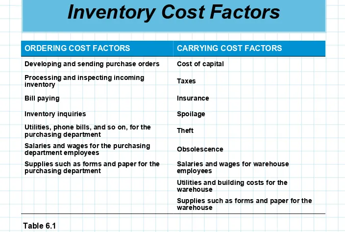
Inventory Cost Factors
ORDERING COST FACTORS CARRYING COST FACTORS
Developing and sending purchase orders Cost of capital
Processing and inspecting incoming
inventory Taxes
Bill paying Insurance
Inventory inquiries Spoilage
Utilities, phone bills, and so on, for the
purchasing department Theft Salaries and wages for the purchasing
department employees Obsolescence Supplies such as forms and paper for the
purchasing department Salaries and wages for warehouse employees Utilities and building costs for the warehouse
Supplies such as forms and paper for the warehouse
Inventory Cost Factors
Ordering costs are generally independent
of order quantity
Many involve personnel time
The amount of work is the same no matter the
size of the order
Carrying costs generally varies with the
amount of inventory, or the order size
The labor, space, and other costs increase as
the order size increases
Of course, the actual cost of items
© 2009 Prentice-Hall, Inc. 6 – 14
Economic Order Quantity
The
economic order quantity
economic order quantity
(
EOQ
EOQ
)
model is one of the oldest and most
commonly known inventory control
techniques
It dates from a 1915 publication by
Ford W. Harris
It is still used by a large number of
organizations today
It is easy to use but has a number of
Economic Order Quantity
Assumptions
1. Demand is known and constant
2. Lead time (the time between the placement and
receipt of an order) is known and constant
3. Receipt of inventory is instantaneous
Inventory from an order arrives in one batch, at
one point in time
4. Purchase cost per unit is constant throughout
the year; no quantity discounts
5. The only variable costs are the placing an order,
ordering cost
ordering cost, and holding or storing inventory over time, holding or holding carrying cost, and these are carrying cost
constant throughout the year
6. Orders are placed so that stockouts or shortages
© 2009 Prentice-Hall, Inc. 6 – 16
Inventory Usage Over Time
Time Inventory
Level
Minimum Inventory
0
Order Quantity = Q =
Maximum Inventory Level
Figure 6.2
Inventory usage has a sawtooth shape
Inventory jumps from 0 to the maximum when the shipment arrivesEOQ Inventory Costs
The objective is to minimize total costs
The relevant costs are the ordering and carrying/
holding costs, all other costs are constant. Thus, by
minimizing the sum of the ordering and carrying costs, we are also minimizing the total costs
The annual ordering cost is the number of orders per
year times the cost of placing each order
As the inventory level changes daily, use the average
inventory level to determine annual holding or carrying cost
The annual carrying cost equals the average inventory
times the inventory carrying cost per unit per year
The maximum inventory is Q and the average inventory
© 2009 Prentice-Hall, Inc. 6 – 18
Inventory Costs in the EOQ Situation
Objective is generally to minimize total cost
Relevant costs are ordering costs and carrying
costs
2 level
inventory
Average Q
INVENTORY LEVEL
DAY BEGINNING ENDING AVERAGE
April 1 (order received) 10 8 9
April 2 8 6 7
April 3 6 4 5
April 4 4 2 3
April 5 2 0 1
Maximum level April 1 = 10 units
Total of daily averages = 9 + 7 + 5 + 3 + 1 = 25 Number of days = 5
Inventory Costs in the EOQ Situation
Develop an expression for the ordering cost.
Develop and expression for the carrying cost.
Set the ordering cost equal to the carrying
cost.
Solve this equation for the optimal order
© 2009 Prentice-Hall, Inc. 6 – 20
Inventory Costs in the EOQ Situation
Mathematical equations can be developed using
Q = number of pieces to order
EOQ = Q* = optimal number of pieces to order
D = annual demand in units for the inventory item
Co = ordering cost of each order
Ch = holding or carrying cost per unit per year
Annual ordering cost
Inventory Costs in the EOQ Situation
Mathematical equations can be developed using
Q = number of pieces to order
EOQ = Q* = optimal number of pieces to order
D = annual demand in units for the inventory item
Co = ordering cost of each order
Ch = holding or carrying cost per unit per year
h
C Q
2
Annual holding cost inventoryAverage
Carrying cost per unit
per year
Total Inventory Cost =
C
oQ
C
hQ
D
2
© 2009 Prentice-Hall, Inc. 6 – 22
Inventory Costs in the EOQ Situation
Minimum Total Cost
Optimal Order Quantity
Curve of Total Cost
Curve of Total Cost
of Carrying
of Carrying
and Ordering
and Ordering
Carrying Cost Curve
Carrying Cost Curve
Ordering Cost Curve
Ordering Cost Curve
Cost
Order Quantity
Figure 6.3
Finding the
EOQ
When the EOQ assumptions are met, total cost is
minimized when Annual ordering cost = Annual holding cost h o C Q C Q D 2
Solving for Q
h o Q C
© 2009 Prentice-Hall, Inc. 6 – 24
Economic Order Quantity (EOQ) Model
h
C Q
2 cost
holding
Annual
o
C Q
D
cost ordering
Annual
h o
C DC Q 2
*
EOQ
Sumco Pump Company Example
Company sells pump housings to other
companies
Would like to reduce inventory costs by finding
optimal order quantity
Finding Total Annual Cost
Annual demand = 1,000 units Ordering cost = $10 per order
© 2009 Prentice-Hall, Inc. 6 – 26
Sumco Pump Company Example
Total annual cost = Order cost + Holding cost
h o C Q C Q D TC 2 ) . ( ) ( , 5 0 2 200 10 200 000 1 100 50
50 $ $
$
© 2009 Prentice-Hall, Inc. 6 – 28
Sumco Pump Company Example
Sumco Pump Company Example
© 2009 Prentice-Hall, Inc. 6 – 30
Purchase Cost of Inventory Items
Total inventory cost can be written to include the
cost of purchased items
Given the EOQ assumptions, the annual
purchase cost is constant at D C no matter the order policy
C is the purchase cost per unit D is the annual demand in units
It may be useful to know the average dollar level
of inventory
2 level
dollar
Purchase Cost of Inventory Items
Inventory carrying cost is often expressed as an
annual percentage of the unit cost or price of the inventory
This requires a new variable
Annual inventory holding charge as a percentage of unit price or cost
I
The cost of storing inventory for one year is then
IC Ch
thus,
IC DC
Q 2 o
© 2009 Prentice-Hall, Inc. 6 – 32
Sensitivity Analysis with the
EOQ Model
The EOQ model assumes all values are know and
fixed over time
Generally, however, the values are estimated or
may change
Determining the effects of these changes is
called sensitivity analysissensitivity analysis
Because of the square root in the formula,
changes in the inputs result in relatively small changes in the order quantity
h o
C DC
2
Sensitivity Analysis with the
EOQ Model
In the Sumco example
units 200 50 0 10 000 1 2 . ) )( , ( EOQ
If the ordering cost were increased four times from
$10 to $40, the order quantity would only double
units 400 50 0 40 000 1 2 . ) )( , ( EOQ
In general, the EOQ changes by the square root
© 2009 Prentice-Hall, Inc. 6 – 34
Reorder Point:
Determining When To Order
Once the order quantity is determined, the next
decision is
when to order
when to order
The time between placing an order and its
receipt is called the
lead time
lead time
(
L
L
) or
delivery
delivery
time
time
Inventory must be available during this period to
met the demand
When to order is generally expressed as a
reorder point
reorder point
(
ROP
ROP
) – the inventory level at
which an order should be placed
Demand
per day new order in daysLead time for a
ROP
Determining the Reorder Point
The slope of the graph is the daily inventory
usage
Expressed in units demanded per day,
d
If an order is placed when the inventory level
© 2009 Prentice-Hall, Inc. 6 – 36
Procomp’s Computer Chip Example
Demand for the computer chip is 8,000 per year Daily demand is 40 units
Delivery takes three working days
ROP d L 40 units per day 3 days 120 units
An order is placed when the inventory reaches
120 units
The order arrives 3 days later just as the
The Reorder Point (ROP) Curve
In
ve
nt
or
y
L
ev
el
(
U
ni
ts
)
Q
*
ROP
(Units)
Slope = Units/Day = d
© 2009 Prentice-Hall, Inc. 6 – 38
EOQ Without The
Instantaneous Receipt Assumption
When inventory accumulates over time, the
instantaneous receipt
instantaneous receipt assumption does not apply
Daily demand rate must be taken into account
The revised model is often called the production production
run model
run model
Inventory Level
Time Part of Inventory Cycle
Part of Inventory Cycle
During Which Production is
During Which Production is
Taking Place
Taking Place
There is No Production
There is No Production
During This Part of the
During This Part of the
EOQ Without The
Instantaneous Receipt Assumption
Instead of an ordering cost, there will be a
setup cost
–
the cost of setting up the
production facility to manufacture the desired
product
Includes the salaries and wages of employees
who are responsible for setting up the
equipment, engineering and design costs of
making the setup, paperwork, supplies,
utilities, etc.
The optimal production quantity is derived by
© 2009 Prentice-Hall, Inc. 6 – 40
Annual Carrying Cost for
Production Run Model
In production runs, setup cost replaces ordering setup cost
cost
The model uses the following variables
Q number of pieces per order, or production run
Cs setup cost
Ch holding or carrying cost per unit per year
p daily production rate
d daily demand rate
Annual Carrying Cost for
Production Run Model
Maximum inventory level
(Total produced during the production run)
– (Total used during the production run)
(Daily production rate)(Number of days production)
– (Daily demand)(Number of days production)
(pt) – (dt)
since Total produced Q pt
we know t Qp
Maximum inventory
level
© 2009 Prentice-Hall, Inc. 6 – 42
Annual Carrying Cost for
Production Run Model
Since the average inventory is one-half the
Annual Setup Cost for
Production Run Model
s
C Q
D
cost setup
Annual
Setup cost replaces ordering cost when a product is
produced over time (independent of the size of the order and the size of the production run)
and
o
C Q
D
cost ordering
© 2009 Prentice-Hall, Inc. 6 – 44
Determining the Optimal
Production Quantity
By setting setup costs equal to holding costs, we
can solve for the optimal order quantity
Annual holding cost Annual setup cost
s h C Q D C p d Q 1 2
Solving for Q, we get
Production Run Model
Summary of equations
p d C DC Q h s 1 2 quantity production Optimal * s C Q D cost setup Annual h C p d Q 1 2 cost holding Annual
© 2009 Prentice-Hall, Inc. 6 – 46
Brown Manufacturing Example
Brown Manufacturing produces commercial
refrigeration units in batches
Annual demand D 10,000 units Setup cost Cs $100
Carrying cost Ch $0.50 per unit per year Daily production rate p 80 units daily
Daily demand rate d 60 units daily
How many refrigeration units should Brown produce in each batch?
Brown Manufacturing Example
p d C DC Q h s 1 2 * 1. 2. 80 60 1 5 0 100 000 10 2 . , * Q© 2009 Prentice-Hall, Inc. 6 – 48
Brown Manufacturing Example
Brown Manufacturing Example
© 2009 Prentice-Hall, Inc. 6 – 50
Quantity Discount Models
Quantity discounts are commonly available
The basic EOQ model is adjusted by adding in the
purchase or materials cost
Total cost Material cost + Ordering cost + Holding cost
h o C
Q C
Q D DC
2 cost
Total
where
D annual demand in units
Cs ordering cost of each order
C cost per unit
Ch holding or carrying cost per unit per year Holding cost Ch IC
© 2009 Prentice-Hall, Inc. 6 – 52
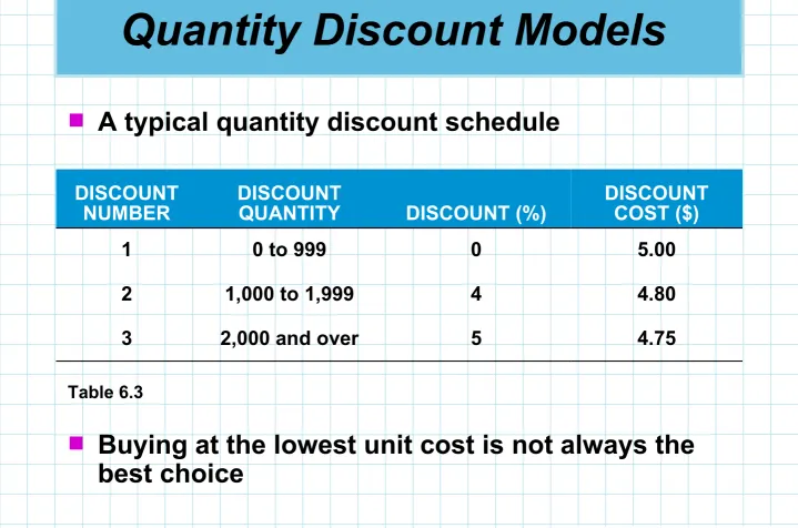
Quantity Discount Models
A typical quantity discount schedule
DISCOUNT
NUMBER DISCOUNT QUANTITY DISCOUNT (%) DISCOUNT COST ($)
1 0 to 999 0 5.00
2 1,000 to 1,999 4 4.80
3 2,000 and over 5 4.75
Table 6.3
Buying at the lowest unit cost is not always the
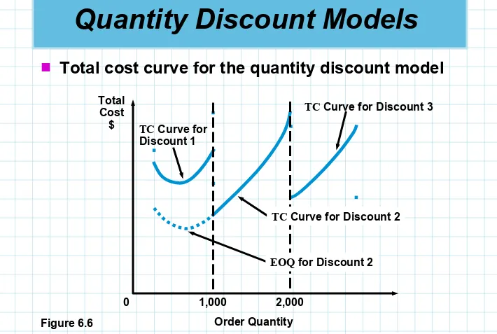
Quantity Discount Models
Total cost curve for the quantity discount model
Figure 6.6
TC Curve for Discount 1
TC Curve for Discount 3 Total
Cost $
Order Quantity
0 1,000 2,000
TC Curve for Discount 2
© 2009 Prentice-Hall, Inc. 6 – 54
Brass Department Store Example
Brass Department Store stocks toy race cars Their supplier has given them the quantity
discount schedule shown in Table 6.3
Annual demand is 5,000 cars, ordering cost is $49, and
holding cost is 20% of the cost of the car
The first step is to compute EOQ values for each
discount order per cars 700 00 5 2 0 49 000 5 2
1
) . )( . ( ) )( , )( ( EOQ order per cars 714 80 4 2 0 49 000 5 2
2
) . )( . ( ) )( , )( ( EOQ order per cars 718 75 4 2 0 49 000 5 2
3
Brass Department Store Example
The second step is adjust quantities below the
allowable discount range
The EOQ for discount 1 is allowable
The EOQs for discounts 2 and 3 are outside the
allowable range and have to be adjusted to the smallest quantity possible to purchase and
receive the discount
Q1 700
Q2 1,000
© 2009 Prentice-Hall, Inc. 6 – 56
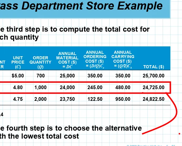
Brass Department Store Example
The third step is to compute the total cost for
each quantity
DISCOUNT NUMBER
UNIT PRICE
(C)
ORDER QUANTITY
(Q)
ANNUAL MATERIAL
COST ($) = DC
ANNUAL ORDERING
COST ($) = (D/Q)Co
ANNUAL CARRYING
COST ($)
= (Q/2)Ch TOTAL ($)
1 $5.00 700 25,000 350.00 350.00 25,700.00
2 4.80 1,000 24,000 245.00 480.00 24,725.00
3 4.75 2,000 23,750 122.50 950.00 24,822.50
The fourth step is to choose the alternative
with the lowest total cost
Brass Department Store Example
© 2009 Prentice-Hall, Inc. 6 – 58
Brass Department Store Example
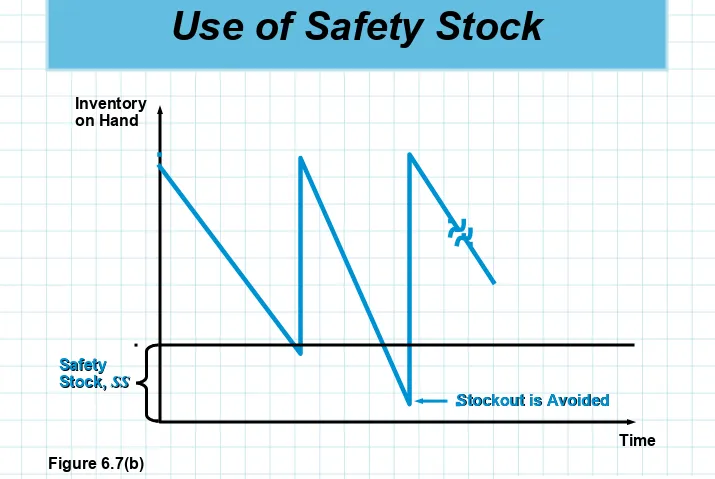
Use of Safety Stock
If demand or the lead time are uncertain,
the exact
ROP
will not be known with
certainty
To prevent
stockouts
stockouts
, it is necessary to
carry extra inventory called
safety stock
safety stock
Safety stock can prevent stockouts when
demand is unusually high
Safety stock can be implemented by
© 2009 Prentice-Hall, Inc. 6 – 60
Use of Safety Stock
The basic ROP equation is ROP d L
d daily demand (or average daily demand)
L order lead time or the number of working days it takes to deliver an order (or average lead time)
A safety stock variable is added to the equation
to accommodate uncertain demand during lead time
ROP d L + SS
where
Use of Safety Stock
Stockout
Stockout
Figure 6.7(a) Inventory on Hand
© 2009 Prentice-Hall, Inc. 6 – 62
Use of Safety Stock
Figure 6.7(b) Inventory on Hand
Time Stockout is Avoided
Stockout is Avoided
Safety
Safety
Stock,
Just-in-Time Inventory Control
To achieve greater efficiency in the
production process, organizations have
tried to have less in-process inventory on
hand
This is known as
JIT inventory
JIT inventory
The inventory arrives just in time to be
used during the manufacturing process
One technique of implementing JIT is a
© 2009 Prentice-Hall, Inc. 6 – 64
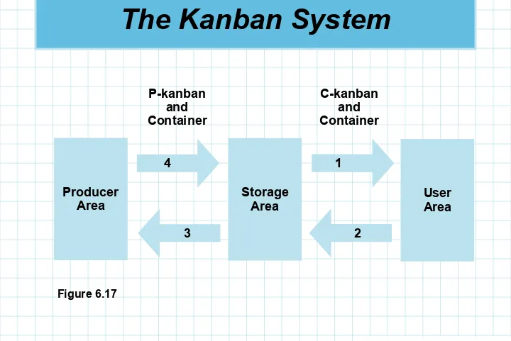
Just-in-Time Inventory Control
Kanban in Japanese means “card”
With a dual-card kanban system, there is a
conveyance kanban, or C-kanban, and a
production kanban, or P-kanban
Kanban systems are quite simple, but they
require considerable discipline
Supplier or the warehouse delivers
components to the production line only as and
when they are needed
Production lines only produce/deliver desired
components when they receive a card and an
empty container, indicating that more parts will
be needed in production
As there is little inventory to cover variability,
4 Steps of Kanban
1. A user takes a container of parts or inventory
along with its C-kanban to his or her work area When there are no more parts or the container is empty, the user returns the container along with the C-kanban to the producer area
2. At the producer area, there is a full container of
parts along with a P-kanban
© 2009 Prentice-Hall, Inc. 6 – 66
4 Steps of Kanban
3. The detached P-kanban goes back to the
producer area along with the empty container
The P-kanban is a signal that new parts are to be manufactured or that new parts are to be placed in the container and is attached to the container when it is filled
4. This process repeats itself during the typical
The Kanban System
Producer
Area Storage Area User Area
P-kanban and Container
C-kanban and Container
4
3 2
1
© 2009 Prentice-Hall, Inc. 6 – 68
Dependent Demand: The Case for
Material Requirements Planning
All the inventory models discussed so far have
assumed demand for one item is independent
of the demand for any other item
However, in many situations items demand is
dependent on demand for one or more other
items
In these situations,
MRP
MRP
can be employed
effectively
Material Requirements Planning (MRP) is an
inventory model that can handle dependent
demand
Dependent Demand: The Case for
Material Requirements Planning
Some of the benefits of MRP are
1. Increased customer service levels 2. Reduced inventory costs3. Better inventory planning and scheduling 4. Higher total sales
5. Faster response to market changes and shifts 6. Reduced inventory levels without reduced
customer service
Most MRP systems are computerized, but
© 2009 Prentice-Hall, Inc. 6 – 70
Structure of the MRP System
Output Reports Output Reports MRP by period report MRP by date report Planned order report Purchase advice Exception reports Order early or late
or not needed Order quantity too
small or too large Data Files
Data Files
Purchasing data BOM
Lead times (Item master file)
MRP has evolved to include not only the materials
required in production, but also the labor hours, material cost, and other resources related to
production
In this approach the term MRP II is often used and
the word resourceresource replaces the word requirementsrequirements
As this concept evolved and sophisticated
software was developed, these systems became known as enterprise resource planning enterprise resource planning (ERPERP) systems
© 2009 Prentice-Hall, Inc. 6 – 72
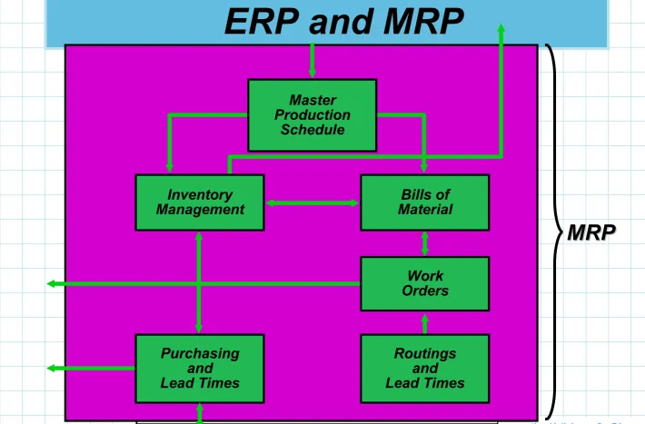
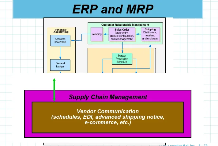
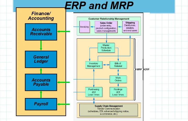
ERP and MRP
Customer Relationship Management
Invoicing
Shipping Distributors,
retailers, and end users Sales Order
(order entry,
© 2009 Prentice-Hall, Inc. 6 – 74
Table 13.6
Bills of Material
Work Orders
Purchasing and Lead Times
Routings and Lead Times Master
Production Schedule
Inventory Management
MRP MRP
Figure 14.11
Supply Chain Management
Vendor Communication
(schedules, EDI, advanced shipping notice, e-commerce, etc.)
© 2009 Prentice-Hall, Inc. 6 – 76
Figure 14.11Table 13.6
Finance/ Accounting
General Ledger Accounts Receivable
Payroll Accounts
Payable
The objective of an ERP System is to reduce costs
by integrating all of the operations of a firm
Starts with the supplier of materials needed and
flows through the organization to include invoicing the customer of the final product
Data are entered only once into a database where
it can be quickly and easily accessed by anyone in the organization
Benefits include
Reduced transaction costs
Increased speed and accuracy of information
Almost all areas of the firm benefit
© 2009 Prentice-Hall, Inc. 6 – 78
There are drawbacks
The software is expensive to buy and
costly to customize
Small systems can cost hundreds of thousands
of dollars
Large systems can cost hundreds of millions
The implementation of an ERP system may
require a company to change its normal
operations
Employees are often resistant to change
Training employees on the use of the new
software can be expensive
The most common ones are from the firms
SAP,
Oracle,
People Soft,
Baan, and
JD Edwards.
Even small systems can cost hundreds of
thousands of dollars.
The larger systems can cost hundreds of millions
of dollars.