Instantaneous Deteriorated Economic Order
Quantity (EOQ) Model with Promotional Effort
Cost
Padmabati Gahan
1, Sourav Dhal
2, Monalisha Pattnaik
3*1,3Dept. of Business Administration, Sambalpur University, Jyotivihar, Sambalpur, India 2Cluster Supply Planner, Hindustan Coca Cola Beverage Pvt. Ltd., Bengaluru, Karnataka, India Abstract—This model studies the problem by proposing a
continuous review inventory model under promotion by assuming that the units do not lost due to deterioration of the items. In this model optimization has been studied for applying promotional effort cost with promotion constraint. The effect of deteriorating items on the instantaneous profit maximization replenishment model under promotion is considered in this model. The market demand may increase with the promotion of the product over time when the units do not lost due to deterioration. In this model, promotional effort and replenishment decision are adjusted arbitrarily upward or downward for profit maximization model in response to the change in market demand within the planning horizon with fixed ordering cost. The objective of this model is to determine the optimal time length, the promotional effort and the replenishment quantity with fixed ordering cost so that the net profit is maximized and the numerical analysis show that an appropriate promotion policy can benefit the retailer and that promotion policy is important, especially for deteriorating items. Finally, sensitivity analyses of the optimal solution with respect to the major parameters are also studied to draw the managerial implications.
Keywords— Instantaneous production, Promotional effort cost, Deteriorated items, Profit maximization model.
I. INTRODUCTION
Inventory management plays a significant role in businesses since it can help the companies to reach the goal ensuring prompt delivery, avoiding shortages, helping sales at competitive prices with cost effective and efficiency. Inventory management is one of the most important components of the production function where the production function is the mid between procurement function and physical distribution function. Since inventory management is the key factor of the production function so,
success of production system in a company. The mission of inventory management are the right quality, the right quantity, the right condition, the right cost tradeoffs, the right customer, the right information, the right response, the right time, the right value, the right product and the right place. The mathematical modeling of real-world inventory problems necessitates the simplification of assumptions to make the mathematics flexible. However, excessive simplification of assumptions results in mathematical models that do not represent the inventory situation to be analyzed. Many models have been proposed to deal with a variety of inventory problems. The classical analysis of inventory control considers three costs for holding inventories. These costs are the ordering cost, carrying cost and shortage cost. The classical analysis builds a model of an inventory system and calculates the EOQ which minimize these three costs so that their sum is satisfying minimization criterion. One of the unrealistic assumptions is that items stocked preserve their physical characteristics during their stay in inventory. Items in stock are subject to many possible risks, e.g. damage, spoilage, dryness; vaporization etc., those results decrease of usefulness of the original one and a cost is incurred to account for such risks. To control an inventory system, one cannot be ignored demand since inventory is partially determined by demand, as suggested by Waters (1994) and Osteryoung, Mc Carty and Reinhart (1986) in many cases a small change in the demand pattern may result in a large change in optimal inventory decisions. A manager of a company has to investigate the factors that influence demand pattern,
of retail inventory is assumed to have a motivating effect on the customer.
Many models have been proposed to deal with a variety of inventory problems. Comprehensive reviews of inventory models can be found in Rafaat (1991) and Jain and Silver (1994). Pattnaik (2012) derived some deterministic inventory models, which are developed under the assumption that demand is either constant or stock dependent for deteriorated items. Bose, Goswami and Chaudhuri (1995) dealt with the EOQ problem for deteriorating items with linear time dependent demand rate under inflation where shortages and discounts are allowed. Goyal and Gunasekaran (1995) considered the effect of different market policies, e.g. the price per product and advertisement frequency on the demand of a perishable item. Gupta and Gerchak (1995) analyzed two scenarios; the first considers TOD as a constant and the store manager may choose an appropriate value, while the second assumes that TOD is a random variable. Hariga (1995) proposed the correct theory for the problem supplied with numerical examples. The most recent work found in the literature is that of Hariga (1996) who extended his earlier work by assuming a time-varying demand over a finite planning horizon. Padmabhan and Vrat (1995) presented an EOQ inventory model for perishable items with a stock dependent selling rate. Unlike the work of Wee (1993) who studied the case of partial backlogging for deteriorating items, Salameh, Jaber and Noueihed (1999) studied an EOQ inventory model in which it assumes that the percentage of on-hand inventory wasted due to deterioration is a characteristic feature of the inventory conditions which govern the item stocked.
Furthermore, retailer promotional activity has become more
and more common in today’s business world. For example,
Wall Mart and Costco often try to stimulate demand for specific types of electric equipment by offering price discounts; clothiers Baleno and NET make shelf space for specific clothes items available for longer periods;
McDonald’s and Burger King often use coupons to attract
consumers. Other promotional strategies include free goods, advertising, and displays and so on. The promotion policy is very important for the retailer. How much promotional effort the retailer makes has a big impact on annual profit. Residual costs may be incurred by too many promotions
while too few may result in lower sales revenue. Tsao and Sheen (2008) discussed dynamic pricing, promotion and replenishment policies for a deteriorating item under permissible delay in payment. Hariga (1994) studied the effects of inflation and time value of money on the replenishment policies of items with time continuous non-stationary demand over a finite planning horizon.
This study addresses the problem by proposing a continuous review inventory model under promotion by assuming that the units do not lost due to deterioration of the items. In this model optimization has been studied for applying promotional effort cost with promotion constraint. The effect of deteriorating items on the instantaneous profit maximization replenishment model under promotion is considered in this model. The market demand may increase with the promotion of the product over time when the units do not lost due to deterioration. In the existing literature about promotion it is assumed that the promotional effort cost is a function of promotion. Tripathy and Pattnaik (2008, 2011) studies profit maximization entropic order quantity model for deteriorated items with stock dependent demand where discounts are allowed for acquiring more profit. In this model, promotional effort and replenishment decision are adjusted arbitrarily upward or downward for profit maximization model in response to the change in market demand within the planning horizon. The objective of this model is to determine optimal promotional efforts and replenishment quantities in an instantaneous replenishment profit maximization model.
Table.1: Summary of the Related Researches
Time and Price Linear and Decreasing development of the model. The mathematical formulation is developed in Section 3. The solution procedure is given in Section 4. In Section 5, numerical example is presented to illustrate the development of the model. The sensitivity analysis is carried out in Section 6 to observe the changes in the optimal solution. Finally in Section 7 the summary and the concluding remarks are explained.
II. ASSUMPTIONS AND NOTATIONS
r Consumption rate, tc Cycle length,
h Holding cost of one unit for one unit of time, HC (q) Holding cost per cycle,
c Purchasing cost per unit, Ps Selling Price per unit,
α Percentage of on-hand inventory that is lost due to deterioration,
q Order quantity,
� Ordering cost per cycle,
q* Traditional economic ordering quantity (EOQ), The promotional effort per cycle
Denote (t) as the on-hand inventory level at time t. During a change in time from point t to t+dt, where t + dt > t, the It is a differential equation, solution is
t =−α + q + α × e−αt
Where q is the order quantity which is instantaneously replenished at the beginning of each cycle of length tc units
Fig.1: Behavior of the Inventory over a Cycle for a Deteriorating Item
Equation t and t are used to develop the mathematical
model. It is worthy to mention that as α approaches to zero, � approaches to . The total cost per cycle, TC (q, ) is the
Hence the profit maximization problem is: Maximize 1 (q, )
∀ ≥ , ≥
IV. OPTIMIZATION
The optimal ordering quantity q per cycle can be determined by differentiating equation , with respect to q, then setting these to zero.
In order to show the uniqueness of the solution in, it is sufficient to show that the net profit function throughout the cycle is concave in terms of ordering quantity q. The second order derivates of the equation , with respect to q are strictly negative. Consider the following propositions.
Proposition 1 The net profit , ) per cycle is concave downward or convex upward in q. Conditions for optimal q is
= � − − ℎ = The second order derivative of the net profit per cycle with
respect to q can be expressed as: = − ℎ that the determinant of the Hessian matrix is positive, i.e.
The objective is to determine the optimal values of q to maximize the unit profit function of , . It is very difficult to derive the optimal values of q, hence unit profit function. There are several methods to cope with constraints optimization problem numerically. But here LINGO 13.0 software is used to derive the optimal values of the decision variable.
V. NUMERICAL EXAMPLE
Consider an inventory situation where K is Rs. 200 per order, h is Rs. 5 per unit per unit of time, r is 1000 units per unit of time, c is Rs. 100 per unit, the selling price per unit
Ps is Rs. 125, � is 0%, � = . and � =1.0. The optimal
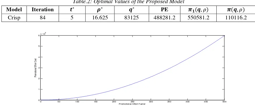
solution that maximizes , , ∗ and ∗are determined by using LINGO 13.0 version software and the results are tabulated in Table 2. Fig. 2 represents two dimensional plotting of promotional effort factor and promotional effort cost PE. Fig. 3 is the three dimensional mesh plot of order quantity q, cycle length � and net profit per cycle . Fig. 4 is the sensitivity plotting of cycle length � , order quantity q and net profit per cycle , .
The optimal solution that maximizes , and ∗are determined by using LINGO 13.0 version software and the results are tabulated in Table 2.
Table.2: Optimal Values of the Proposed Model
Model Iteration �∗ ∗ �∗ PE � �, �,
Crisp 84 5 16.625 83125 488281.2 550581.2 110116.2
Fig.2: Two Dimensional Plotting of Promotional Effort Factor and Promotional Effort Cost PE
Fig.3: Three Dimensional Mesh Plotting of Order Quantity q, Promotional Effort Factor and Net Profit per Cycle ,
0 50 100 150 200 250 300 350 400 450 500
0 1 2 3 4 5 6x 10
8
Promotional Effort Factor
P
ro
m
o
ti
o
n
a
l
E
ff
o
rt
C
o
s
Fig.4: Sensitivity Plotting of Order Quantity q, Promotional Effort Cost PE and Net Profit per Cycle ,
VI. SENSITIVITY ANALYSIS
It is interesting to investigate the influence of the major parameters K, h, r, c and � retailer’s behavior. The computational results shown in Table 3 indicate the following managerial phenomena:
� the replenishment cycle length, q the optimal replenishment quantity, the promotional effort factor, PE promotional effort cost, the optimal net profit per unit per cycle and the optimal average profit per unit per cycle are insensitive to the parameter K.
� the replenishment cycle length, q the optimal replenishment quantity, the promotional effort factor, PE promotional effort cost, the optimal net profit per unit per cycle and the optimal average profit per unit per cycle are moderately sensitive to the parameter h.
q the optimal replenishment quantity, PE promotional effort cost, the optimal net profit per unit per cycle and the optimal average profit per unit per cycle are sensitive to the parameter r but � the replenishment cycle length and the promotional effort factor is insensitive to the parameter r.
� the replenishment cycle length, q the optimal replenishment quantity, the promotional effort factor, PE promotional effort cost, the optimal net profit per unit per cycle and the optimal average profit per unit per cycle are insensitive to the parameter c.
� the replenishment cycle length, q the optimal replenishment quantity, the promotional effort factor, PE promotional effort cost, the optimal net profit per unit per cycle and the optimal average profit per unit per cycle are insensitive to the parameter �.
Table.3: Sensitivity Analyses of the parameters K, h, r, c and �
Parameter Value Iteration �∗ �∗ ∗ PE � �, �, % Change
in � �,
K
201 88 5 83125 16.63 488281.2 550580.2 110116.0 0.00018 205 82 5 83125 16.63 488281.2 550576.2 110115.2 0.00091 208 87 5 83125 16.63 488281.3 550573.3 110114.6 0.00143 h
5.1 95 4.90 79993.27 16.32 469320.7 530395.2 108200.6 3.66631 5.2 87 4.81 77038.65 16.02 451443.5 511339.6 106358.6 7.12730 5.5 95 4.55 69111.57 15.20 403538.2 406156.4 101234.4 26.2313 r
1050 91 5 87281.25 16.63 512695.3 578120.3 115624.1 5.00182 1040 93 5 86450.00 16.63 507812.5 572612.5 114522.5 4.00146 1060 96 5 88112.50 16.63 517578.1 583628.1 116725.6 78.7996 c
105 77 4 44000 11.00 200000.0 239800.0 59950.0 56.4460 90 98 7 221375 31.63 1875781 1998081.0 285440.2 262.904 110 100 3 19875 6.63 63281.25 85581.25 28527.08 84.4562
�
VII. CONCLUSION
In this model, a traditional EOQ model is introduced which investigates the optimal order quantity assumes that the inventory conditions govern the item stocked for general case. This model provides a useful property for finding the optimal profit and ordering quantity where the deteriorated units are not lost. A mathematical EOQ model is developed and satisfied the properties numerically. The economic order quantity and the net profit for the present model were found to be optimum respectively. Further, a numerical example is presented to illustrate the theoretical results, and some observations are obtained from sensitivity analyses with respect to the major parameters to draw the managerial implications. The model in this study is a general framework in crisp decision space.
In the future study, it is hoped to further incorporate the proposed models into several situations such as shortages are allowed and the consideration of multi-item problem. Furthermore, it may also take partial backlogging into account when determining the optimal replenishment policy. There are many scopes in extending the present work as a future research work. Parameters and decision variables can be considered random or even fuzzy. Effect of shortage, backlogging inflation etc could be added to the multi-item model. The current work can be extended in order to incorporate the modified model with shortages are allowed and the consideration of multi-item problem. A further issue that is worth exploring is that of partial backlogging. Finally, few additional aspects that the near future are the applying dynamic pricing strategy are intended through a new optimization model and stochastically of the quality of the products.
REFERENCES
[1] Bose, S., Goswami, A. and Chaudhuri, K.S. “An EOQ model for deteriorating items with linear time-dependent demand rate and shortages under inflation
and time discounting”. Journal of Operational Research Society, 46: 775-782, 1995.
[2] Goyal, S.K. and Gunasekaran, A. “An integrated production-inventory-marketing model for
deteriorating items”. Computers and Industrial Engineering, 28: 755-762, 1995.
[3] Gupta, D. and Gerchak, Y. “Joint product durability
and lot sizing models”. European Journal of Operational Research, 84: 371-384, 1995.
[4] Hariga, M. “Economic analysis of dynamic inventory models with non-stationary costs and demand”.
International Journal of Production Economics, 36: 255-266, 1994.
[5] Hariga, M. “An EOQ model for deteriorating items with shortages and time-varying demand”. Journal of Operational Research Society, 46: 398-404, 1995. [6] Hariga, M. “An EOQ model for deteriorating items
with time-varying demand”. Journal of Operational Research Society, 47: 1228-1246, 1996.
[7] Jain, K. and Silver, E. “A lot sizing for a product
subject to obsolescence or perishability”. European Journal of Operational Research, 75: 287-295, 1994. [8] Mishra, V.K. “Inventory model for time dependent
holding cost and deterioration with salvage value and shortages”. The Journal of Mathematics and Computer Science, 4(1): 37-47, 2012.
[9] Osteryoung, J.S., Mc Carty, D.E. and Reinhart, W.L.
“Use of EOQ models for inventory analysis”.
Production and Inventory Management, 3rd Qtr: 39-45,
1986.
[10]Padmanabhan, G. and Vrat, P. “EOQ models for
perishable items under stock dependent selling rate”.
European Journal of Operational Research, 86: 281-292, 1995.
[11]Pattnaik, M. “An entropic order quantity (EnOQ) model under instant deterioration of perishable items with price discounts”. International Mathematical Forum, 5(52): 2581-2590, 2010.
[12]Pattnaik, M. “A note on non linear optimal inventory policy involving instant deterioration of perishable
items with price discounts”. The Journal of Mathematics and Computer Science, 3(2): 145-155, 2011.
[13]Pattnaik, M. “Decision-making for a single item EOQ model with demand-dependent unit cost and dynamic
setup cost”. The Journal of Mathematics and Computer Science, 3(4): 390-395, 2011.
[14]Pattnaik, M. “Entropic order quantity (EnOQ) model under cash discounts”. Thailand Statistician Journal, 9(2): 129-141, 2011.
[15]Pattnaik, M. “A note on non linear profit -maximization entropic order quantity (EnOQ) model for deteriorating items with stock dependent demand
rate”. Operations and Supply Chain Management, 5(2): 97-102, 2012.
[16]Pattnaik, M. “An EOQ model for perishable items
with constant demand and instant Deterioration”.
Decision, 39(1): 55-61, 2012.
[18]Pattnaik, M. “The effect of promotion in fuzzy optimal replenishment model with units lost due to
deterioration”. International Journal of Management Science and Engineering Management, 7(4): 303-311, 2012.
[19]Pattnaik, M. “Fuzzy NLP for a Single Item EOQ Model with Demand – Dependent Unit Price and
Variable Setup Cost”. World Journal of Modeling and Simulations, 9(1): 74-80, 2013.
[20]Pattnaik, M. “Linear programming problems in fuzzy
environment: the post optimal analyses”. Journal of Uncertain Systems, in press, 2013.
[21]Pattnaik, M. “Wasting of percentage on-hand inventory of an instantaneous economic order quantity
model due to deterioration”. The Journal of Mathematics and Computer Science, 7: 154-159, 2013.
[22]Raafat, F. “Survey of literature on continuously deteriorating inventory models”. Journal of Operational Research Society, 42: 89-94, 1991. [23]Roy, T.K. and Maiti, M. “A Fuzzy EOQ model with
demand dependent unit cost under limited storage
capacity”. European Journal of Operational Research, 99: 425 – 432, 1997.
[24]Salameh, M.K., Jaber, M.Y. and Noueihed, N. “Effect of deteriorating items on the instantaneous
replenishment model”. Production Planning and Control, 10(2): 175-180, 1993.
[25]Tripathy, P.K., Pattnaik, M. and Tripathy, P.K.
“Optimal EOQ Model for Deteriorating Items with
Promotional Effort Cost”. American Journal of Operations Research, 2(2): 260-265, 2012.
[26]Tripathy, P.K., Pattnaik, M. and Tripathy, P.K. “A Decision-Making Framework for a Single Item EOQ
Model with Two Constraints”. Thailand Statistician Journal, 11(1): 67-76, 2013.
[27]Tsao, Y.C. and Sheen, G.J. “Dynamic pricing, promotion and replenishment policies for a deteriorating item under permissible delay in
payment”. Computers and Operations Research, 35: 3562-3580, 2008.
[28]Waters, C.D.J. “Inventory Control and Management”. (Chichester: Wiley), 1994.
[29]Wee, H.M. “Economic Production lot size model for deteriorating items with partial back-ordering”.