Received December 4, 2015 Published as Economics Discussion Paper December 17, 2015
Distance and Border Effects in International
Trade: A Comparison of Estimation Methods
Glenn Magerman, Zuzanna Studnicka, and Jan Van Hove
Abstract
This paper compares various estimation methods often used in the estimation of gravity models of international trade. The authors first discuss different structural and consistent estimation techniques, their underlying assumptions and their impact on estimated coefficients. They then estimate the gravity model for global bilateral trade flows using various empirical methodologies. They focus on a comparison of the distance and border effects across estimation techniques. For the border effects they take into account adjacency effects as well as the distinction between intra-regional and inter-regional trade. Their findings confirm the significantly negative distance and the significantly positive adjacency effect across estimation methods, although the size of the effects varies substantially across methods. The border effects by global regions are much more sensitive – both in size and direction – to the applied estimation method. Although all estimation methods have their own merits and drawbacks, the authors provide some guidelines for future empirical research based on their findings.
(Published in Special Issue Distance and Border Effects in Economics)
JEL F10 F14
Keywords Gravity model; empirical estimation; distance effect; border effect
Authors
Glenn Magerman, University of Leuven (KU Leuven), Naamsestraat 69, 3000 Leuven, Box 3550, Belgium, [email protected]
Zuzanna Studnicka, ESRI Dublin, Sir John Rogerson’s Quay Dublin 2, Ireland Jan Van Hove, University of Leuven (KU Leuven), Belgium
1
Introduction
“There is very little that economists fully understand about global trade but there is one thing that we do know – commerce declines dramatically with the distance” (Leamer 2007). The negative impact of distance on trade is indeed one of the most robust findings in international economics (e.g. Leamer 1993; Frankel 1997a; Disdier and Head 2008). Moreover, trade does not only decrease in distance, but it is also affected by international borders (McCallum 1995; Wei 1996; Anderson and van Wincoop 2003; Obstfeld and Rogoff 2001; Coughlin and Novy 2012). This leads to two additional robust empirical findings on borders: (i) adjacent countries trade more than non-adjacent countries (see for instance Leamer 1993; Helliwell 1997) and (ii) trade within borders exceeds trade across borders at different levels
of aggregation.
The robust importance of distance and borders as determinants of trade flows can be explained by the variety of barriers to trade they reflect. Distance and border effects are proxies for geographical barriers between trading partners, as well as for various transport costs between partners (see Anderson and van Wincoop (2004) for a survey). On the demand side, geographic distance can also capture consumers’ taste differences, as it reduces trade even in online products, where trade costs are arguably lower than in offline markets (Blum and Goldfarb 2006).
These three well-established empirical results appear in the estimates of the so-called gravity equation and are robust to many different underlying trade models, for instance either assuming perfect competition (Anderson 1979; Deardorff 1995; Eaton and Kortum 2002), monopolistic competition (Bergstrand 1989, 1990) or a demand system with translog preferences (Novy 2013).
elasticity to distance over time (e.g. Leamer 1993). Also Disdier and Head (2008) argue that the distance effect is rather constant after a rise around mid twentieth century. Conversely, Frankel (1997a), Soloaga and Winters (2001), Berthelon and Freund (2008) obtain evidence for an increasing distance effect, whereas e.g. Boisso and Ferrantino (1993), Eichengreen and Irwin (1998), Brun et al. (2005), Felbermayr and Kohler (2006), Coe et al. (2007) observe a negative evolution in the distance effect over time.
There are several possible explanations for these contrasting results. For example, Brun et al. (2005) argue that changes in infrastructure are responsible for the decline of the distance effect. According to Felbermayr and Kohler (2006), the non-decreasing distance effect can be explained when failing to take into account the extensive margin of trade. Conversely, Berthelon and Freund (2008) show that the increase of the overall distance coefficient is due to changes of distance coefficients across industries. They explore two possible reasons for these changes. First, in some industries, goods have become more substitutable. Second, trade costs have changed as well. The authors argue that the first phenomenon is the most important one. Finally, Behar and Venables (2009) argue that the non-decreasing coefficient of distance over time is due to increased trade at shorter distances, relative to that at longer distances.
The empirical literature on border effects was inspired by the seminal work of McCallum (1995), who shows that Canadian provinces trade up to 22 times more with each other than with US states (the so-called home bias). This finding was initially confirmed by Helliwell and McCallum (1995) and Helliwell (1996). Similarly, Wei (1996) finds that OECD countries trade about 2.5 times more internally than with identical foreign countries. Helliwell (1997) points to an even larger border effect, but it is only half for countries sharing a common border and a common language. Following a similar approach as Wei (1996) and Helliwell (1997), Nitsch (2000) finds that domestic trade within a European Union country is seven to ten times larger than trade with another European Union country. Finally, most of these studies observe a trade increasing effect for adjacent countries.
resistance term considerably reduces McCallum’s ratio of inter-provincial trade to province-state trade from 16.4 to 10.7. Additionally, they find that borders reduce trade between the US and Canada by 44% and among other industrialized countries by 29%.
Interestingly, the home bias exists not only at the international level, but also at the intra-national level. According to Wolf (2000), trade between US states is about three times lower than trade within states. Additionally, adjacent states trade 2.6 times more with each other. Strikingly, the distance coefficient is similar to the coefficients found for international trade.
More recently, Coughlin and Novy (2012) compare trade between and within individual US states with trade between states and foreign countries. They find that a state’s border generates a larger trade barrier than an international US border. One possible explanation is related to Hillberry and Hummels (2008) who find that trade within the US is heavily concentrated at the local level: trade within a single ZIP code is on average three times larger than trade with partners outside the ZIP code. Hillberry and Hummels (2008) explain their finding by co-location of producers in supply chains to exploit informational spillovers, minimize transportation costs and facilitate just-in-time production. According to Coughlin and Novy (2012), producers also concentrate in order to benefit from external economies of scale in the presence of intermediate goods and associated agglomeration effects (Rossi-Hansberg 2005), as well as from the hub-and-spoke distribution systems and wholesale shipments (Hillberry and Hummels 2003): the domestic border effect then reflects the local concentration of economic activity rather than trade barriers associated with crossing a state border.
2
The Econometrics of Gravity
2.1 The general gravity equation
While the earliest implementation of the gravity model in international trade was an intuitive copy of its counterpart in physics (Tinbergen 1962), most theoretical trade models now derive an aggregate bilateral demand system that can be written very similar to the physical gravity equation. We can write the gravity equation in general terms as:
Xi j =G
SiMj
φi j
(1)
whereXi j denotes nominal exports from countryito j,Gis a constant,SiandMj
are the capabilities of exporter and importer respectively andφi j is a function of the
impact of trade barriers to bilateral trade flows. Hence, exports fromito j increase
in exporter and importer economic capabilities (e.g. GDP) and decrease in bilateral trade barriers (e.g. geographical distance, tariffs, non-tariff barriers).
Using homothetic budget shares and general equilibrium market clearing under fairly general conditions, one can derive a structural basis for (1) (Costinot and Rodríguez-Clare 2014). Following the model of Anderson and van Wincoop (2003) for instance:
Xi j =
YiEj
PiΠjφi j
(2)
whereYi is gross output of exporter i,Ej is the total expenditure on goods in j
andPiandΠjare multilateral trade resistance terms (MTR), capturing equilibrium
price levels for the exporting and importing country respectively.1
1 Anderson and van Wincoop (2003) useE
i=Yi(balanced trade) to close the model, and enforce
φi j=φji(symmetric trade costs), leading toPi=Πjas a unique solution to the system of equations
Note that we do not suggest time dimensions in this specification, and mainly so for two reasons. First, the bulk of theory in the gravity literature derives static and cross-sectional models from long run equilibrium conditions. Second, most empirics are performed in a panel setting, but in a static way: exploiting the panel dimension allows for time-invariant regressors (such as distance and borders) to infer causation of the model with respect to predicted trade flows. There is a growing literature on “true” dynamic panel models in international trade: see for instance Harris and Matyas (2004); Harris et al. (2009); Baltagi et al. (2014), which we abstract from here.
2.2 Log-linearizing the model and OLS
The parametric specification of the empirical gravity model is assumed to follow the exponential functional form:
Y=exp(Xβ)η (3)
whereXis a vector of regressors with elementsxi j,β is a vector of coefficients
to be estimated, andη is a vector of idiosyncratic error terms so thatE(η|X) =1.
Traditional estimation of the gravity model log-linearizes (3) so that:
y=Xβ+ε (4)
wherey=ln(Y)andε=ln(η). This transformation is often applied in empirical
trade research as it linearizes the estimation equation, allowing for estimators that are straightforward to implement such as OLS to estimate parameters of interest
β. However, this transformation and subsequent estimation with OLS generates
a few important issues related to (i) heteroscedasticity, (ii) zero trade flows and (iii) weights of individual observations in optimally fitting the model. We describe these issues in more detail.
Heteroscedasticity First, the validity of the model depends on the orthogonality
ofε with respect to the regressorsX. When estimating (4), one assumes (among
(
E(ε|X) =0 (strict exogeneity)
E(ε2|X) =σ2(homoscedastic errors)
whereσ >0 is the standard deviation of the errors. However, if the error term is
heteroscedastic, the variance of the error term is not constant(σi6=σ,8i).
One potential cause of heterogeneity is omitted variable bias. If the model is misspecified due to omitted variables or the exclusion of a (non)-linear combination of regressors that are correlated with the error term (violating strict exogeneity), this can lead to a heterogeneous pattern of the residuals.
If heteroscedasticity is moderate, we can transform the estimation equation or use robust methods to correct for the standard errors such as White (1980) standard errors. Also, Weighted Least Squares can be used to account for the heteroscedasticity problem and produce an efficient estimator. However, deriving the correct weighting matrix through iteration can be a tedious task.
Heteroscedasticity does not affect the unbiasedness of the OLS estimator, but it affects the efficiency of the estimator as it does not minimize the variance. It
also affects the estimated p-values and to a lesser extent confidence intervals and
prediction intervals. The estimated standard errors are biased and the bias can go either way. Therefore, other estimators can be more efficient.
account for these structural zeros. Some solutions have been proposed such as se-lection models with a 2-stage estimation procedure, where the first stage estimates the amount of zeros in the system, and the second stage subsequently estimates the bilateral trade values. While Helpman et al. (2008) use a Heckman-type selection model that is derived from theory and accounts for firm heterogeneity, alternatives
such as Zero Inflated models deliver biased results.2
Weights of observations and the loss function Third, different estimators use different weighting schemes and potentially different loss functions in obtaining the optimal fit for the model to produce parameter estimates. Parameter estimates in OLS are obtained by minimizing the Sum of Squared Residuals (SSR), so that:
ˆ
denotes the quadratic loss function. The first-order conditions of the optimization problem are:
∂βˆ
∂ β =−2X
0y+2X0Xβ=0
so that β = (X0X)−1Xy.3 There is a unique minimum if X has full rank (or
equivalently in the absence of perfect multicollinearity – another assumption of the OLS estimator).
The two main candidates for the loss function are the quadratic loss function and the absolute value loss function. OLS uses the quadratic loss function (or least squared errors) which puts larger weight on larger residuals and mainly so for three reasons. First, this loss function generates a unique and stable solution for (5). The
2 Since the Helpman et al. (2008) procedure can only be performed on a small subset of countries
(in order to be computationally able to use fixed effects in a non-linear setting), we do not present the results of those estimations here. In addition, since the count data alternatives of Negative Binomial and Zero Inflated models are biased, we do not go into further details on their estimation in this paper.
3 From the second-order conditions, this is indeed a minimum: ∂2SSR(β)
least absolute deviations regression is more robust to outliers, but it can generate multiple and unstable solutions. Second, as we estimate a conditional mean, the loss function is quadratic by construction. Alternative loss functions result in the estimation of other moments of the data. For instance, a linear loss function results in an estimator equal to a quantile (e.g. median) of the posterior distribution, and an “all-or-nothing” loss function results in the estimation of the mode of the posterior distribution. Third, the quadratic loss function is symmetric, so that positive and negative deviations from the estimated parameter are allocated the same weight.
As an aside, one note on the Maximum Likelihood estimation of (4). In the linear model and under homoscedasticity of the error terms, the first-order
conditions with respect toβ of the objective to be optimized under least squares
and Maximum Likelihood (ML) coincide. In the linear model, the log-likelihood function`(β|X) =−n2ln(2π)−n2ln(σ2)− 1
Instead of log-linearizing (3), we can estimate the coefficients from the model in the original exponential function. Using non-linear least squares (NLS) and optimizing SSR, the objective to estimate parameters of the model becomes:
ˆ
with a system of first-order conditions:
∂βˆ
∂ β =
∑
[Y−exp(Xβ)]exp(Xβ)X=0 (7)The first factor (Y−exp(Xβ)) is the model to be estimated and the factor
exp(Xβ)Xrepresents weights to each observation in minimizing the errors.
equation: this function gives more weight to observations whereexp(Xβ)is large,
so that countries with largerSi andMj for instance, get more weight. There is
economic intuition for this weighting scheme, as countries with higher GDP tend to report more accurately and therefore get more weight in estimating the model. This is not only GDP, but also other variables that might be used in this dimension such as the MTR and the distance function. However, Santos Silva and Tenreyro (2006) state that (i) this does not address the heteroscedasticity problem and (ii) these observations also have the most variance so more noise is added in the model, which brings down the efficiency of the estimation, leading to larger standard errors.
Generally, the estimator could be efficient if one calculates the appropriate weights. This is largely the optimization method Anderson and van Wincoop (2003) propose in their gravity model as in (2). The problem is that the weights have to be calculated together with the MTR for each country pair relative to all other pairs, making this method very cumbersome. To deal with this issue, alternative, non-parametric methods have been proposed (e.g. Robinson 1987). However, empirical researchers enjoy easily implementable methods and have proceeded to
use OLS with a “twist”, or alternatively the PPML method.4
2.4 Least Squares Dummy Variables and Taylor approximation
This twist comes from not having to calculate the NLS procedure, but instead accounting for the non-linear MTR by using exporter and importer fixed effects in the estimation, which can be easily implemented in an OLS estimation. We label this as Least Squares Dummy Variables (LSDV). Anderson and van Wincoop (2003) use the fixed effects approach in one of their procedures, and it is the standard procedure for most empirical researchers using the gravity model.
One drawback of the fixed effects approach is that the system of structural non-linear market clearing conditions of Anderson and van Wincoop (2003) is evaded, and general equilibrium comparative statics are not possible (Baier and
4 While we do not estimate NLS in this paper and focus instead on other non-linear methods
Bergstrand 2009). Additionally – and often more practically – using fixed effects renders identification of variables of interest in those dimensions impossible. One way to accommodate both problems is to approximate the non-linear system by a first-order Taylor approximation, as proposed by Baier and Bergstrand (2009). This allows to account for MTR to an approximation, while having the dimensions of identification free as the researcher sees fit. We label this method as Baier and Bergstrand (BB). The model is then specified as follows:
xi j=β0+β1yi+β2yj+β3lnDisti j⇤+β4Borderi j⇤ +...+εi j (8)
is a first-order Taylor approximation of the non-linearlnDisti j andθiis countryi’s
GDP share in world GDP. The Taylor approximation has to be performed for each bilateral variable of the distance function separately.
2.5 Pseudo Maximum Likelihood Estimators
with first-order conditions:
∂βˆ
∂ β =
∑
[Y−exp(Xβ)]X=0 (11)Santos Silva and Tenreyro (2006) propose to replace the weighting factor of the
original NLS in (7) by an assumption on its behavior. Thenexp(Xβ)X⌘X, i.e.
assuming that weights are proportional to the value of their observations. This satisfies the Poisson model assumption of the conditional mean being proportional to the conditional variance. This is the only assumption taken from the Poisson model, but it happens to coincide with the first-order conditions of the Poisson ML, as seen in (11). If this assumption does not hold in reality however, standard errors are too small.
Note that the starting point of the analysis is NLS. Therefore, no distributional assumptions are made on the model parameters (e.g. the dependent variable does not have to be Poisson distributed), nor is there any other relationship to other count models such as Negative Binomial and Zero-Inflated models.
Notice the difference with (7): each observation is given the same weight now,
xi, rather than emphasizing those for which exp(Xβ)is large as in NLS. These
are not the real first-order conditions of the log likelihood function of the original problem in (7), and therefore are “pseudo”, but they are easier to calculate as the second factor is simplified. Furthermore, Gourieroux et al. (1984) show that these estimators are consistent and asymptotically normal.
Another PML is the Gamma Pseudo ML (GPML), given by:
Pr(Y) =
is the Gamma distribution. In the PPML, we assume equi-dispersion, so that the
variance of the model is proportional to the mean: V(Y X)∝E(Y X). In the
GPML, we assume that the dispersion grows as the observations grow, following
as in OLS and NLS. Both PPML and GPML return consistent estimates, and depending on the variance proportionality, one is more efficient. The first-order conditions are now given by:
∂βˆ
∂ β =
∑
(Y−exp(Xβ))exp(−Xβ)X=0 (13)which is very close to the first-order conditions of NLS, but with different weights.5
2.6 Discussion
Table 1 compares the differences across estimation procedures in terms of weight-ing schemes, dealweight-ing with zeros and heteroscedasticity. First, we consider the differences in weighting schemes. On the one hand, OLS puts more weight on
large deviations through theexp(Xβ)Xweighting scheme. On the other hand, we
can nest the non-linear models as follows. We can write the first-order conditions of NLS, PPML and GPML in vector form as:
∑
(Y−exp(Xβ))[exp(Xβ)]kX=0 (14)where for NLS: k = 1, PPML: k = 0 and GPML: k = −1 respectively, and
[exp(Xβ)]kX represents the weighting scheme of the errors to be minimized.
Hence, from (14), it is immediately visible that NLS gives a weight to devia-tions from the mean proportional to that mean. PPML puts equal weights on all deviations, and GPML allocates weights that are inversely proportional to the mean. Depending on the location of the outliers, this can lead to an upward or downward adjustment of the estimated coefficient.
For instance, consider a toy example with one single outlier in trade-distance space (e.g. one very distant island that trades with only one other country in
5 See also Head and Mayer (2014), who compare first-order conditions of OLS, Poisson true ML
the world). It is easy to imagine the downward sloping regression line in this space. Suppose first that this island trades very little with its partner (so that the observation lies in the North-West of the trade-distance space). Then this outlier will pull the regression line towards itself, leading to a more negative coefficient on distance, and more so for the NLS scheme than the other weighting schemes. However, if this island trades a lot with its partner (now being in the North-East of the trade-distance space), again it will “pull” the coefficient towards itself, but now leading to a less negative coefficient. Considering then that various observations
can be in various locations, makes it clear that it is impossible to predicta priori
the net impact on the size of the estimated coefficient.
Depending on the setting, researchers might then consider which scheme best represents the observed data. For instance, if one assumes that large GDP countries better report GDP values (i.e. with less measurement error), one can opt for the NLS method, so that these countries get more weight in estimating the GDP coefficient of the gravity model. At the same time, the researcher has to be aware that this choice skews the point estimate towards the impact of large GDP countries on bilateral trade flows. Furthermore, this choice simultaneously affects the estimation of all variables, which could involve contrasting interests in the direction of the weighting scheme.
Second, the log-linearized methods of OLS or LSDV/BB do not include zero trade flows. If these zeros are structural (e.g. Helpman et al. 2008), missing flows contain important information on the presence and intensity of exports. While PPML and GPML include zeros in the non-linear estimation, these methods do not structurally account for these zeros. The method described in Helpman et al. (2008) applies a structural and consistent 2-stage estimation method, but its application in typical packages such as STATA – especially for larger samples – is not straightforward as convergence is hard to achieve. Moreover, finding the required exclusion variable for the first stage is arguably difficult. Helpman et al. (2008) use religion as an exclusion variable in their paper.
OLS LSDV/BB PPML GPML
Weights (deviations) More on large More on large Equal weight More on small
Zeros Dropped Dropped In In
Heteroscedasticity Biased standard errors Unbiased Unbiased Unbiased
Table 1:Characteristics estimation procedures
3
Data and Empirical Approach
We use the CEPII/BACI database (Gaulier and Zignago 2010) to create bilateral
trade flows at the country level.6 This is a cleaned and “mirrored”7version of the
UN Comtrade database that records product-level trade at the Harmonised System 6-digit level for almost all countries and economic entities in the world. We convert export values to 1000’s of current US dollars. We aggregate the product-level trade flows to yearly country-level trade flows, drop some accounting aggregates and make some countries that split or merged during the period consistent over time. We extract countries’ nominal GDP in 1000’s of current US dollars from the website of the World Bank.
We obtain indicators such as distance, adjacency, common language and colo-nial ties from the GeoDist database at CEPII as presented by Mayer and Zignago (2011). Distance is recorded as the great circle distance in kilometers between the
most populated cities iniand j. Adjacency is a dummy variable that takes value 1
ifiand jshare a common country border and 0 otherwise. Language is a dummy
that takes value 1 if both countries share an official language. Colony is a dummy
variable that takes value 1 ifiand jever shared a colonial tie.
We use RTA dummies from Jose De Sousa’s website, which are set to 1 if both
countries are in any form of regional trade agreement and 0 otherwise.8 We collect
WTO accession dates from the WTO website to create a duration database of WTO
6 http://www.cepii.com/anglaisgraph/bdd/baci.htm
7 In order to mitigate the potential problem of non-reporting in the data, Gaulier and Zignago (2010)
fill in missing export values with the transpose of the trade matrix, leading to an increase of around 10% observed values in the dataset.
membership. We then generate a dummy for each country equal to 1 if that country
is a member of the WTO in that year.9 Finally, we allocate countries to one of eight
global regions.10 The resulting database covers the years from 1998 to 2011, has
208 countries or economic entities and 602,784 recorded export flows.
We then estimate the gravity specification given by (2) using different estima-tion specificaestima-tions. We apply both linear and non-linear methods. As is common in the gravity literature, we assume that the distance function is linear in
observ-ables, so that:lnφi j =lnDisti j+Ad jacencyi j+Languagei j+Colonyi j+RTAi j+
W T Oi+W T Oj.
4
Results
4.1 Distance coefficient across estimation methods
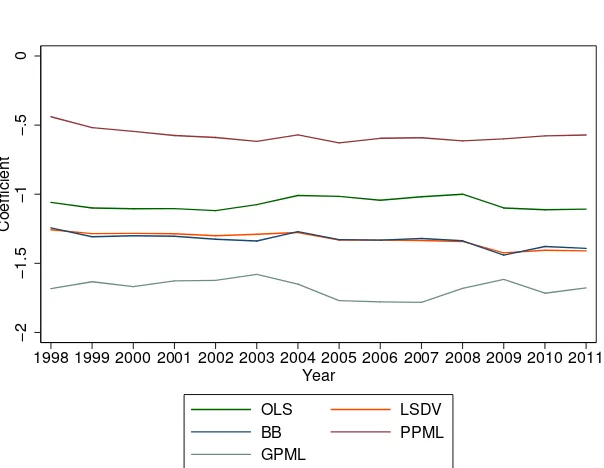
We first analyze the sensitivity of the distance coefficient to the applied estimation techniques. We estimate a series of cross-section gravity models (one for each year between 1998 and 2011), and subsequently plot the coefficients for each year in Figure 1.
The X-axis reports the years 1998 to 2011, the Y-axis plots the estimated coefficients by estimation method. Model specifications are ordinary least squares (OLS), Least Squares Dummy Variable – or OLS with fixed effects (LSDV), Baier and Bergstrand (2009) Taylor approximation method (BB), Poisson Pseudo-Maximum Likelihood (PPML) and Gamma Pseudo-Pseudo-Maximum Likelihood (GPML). The estimated coefficients are reported after correcting for covariates such as GDP and other distance variables explained above. To evade potential endogeneity and
following Baier and Bergstrand (2009), we use simple averages for θi ⌘1/N,
whereN is the number of countries in the sample. A few remarks on the results.
First, all methods confirm the negative and significant effect of distance on export flows. We also confirm that the estimated coefficients are fairly stable over time: the difference of the coefficients in 1998 and 2011 is statistically insignificant
9 http//www.wto.org
10Regions are defined as the following continents and/or global economic regions: Europe, North
at the 1% level for all the estimation methods. However, given the short time span of our data set, we cannot interpret this as evidence for or against the “death of distance” hypothesis described in Section 1.
Second, there is substantial variation in the magnitude of the distance effect across estimation procedures: while the linear procedures OLS, LSDV and BB produce results that are around –1.0 to –1.2, the estimated coefficients using PPML are around –0.5 (in line with the findings of Santos Silva and Tenreyro (2006) and subsequent PPML estimations). The estimated coefficients using GPML are around –1.7.
Third, we see that the LSDV and the BB methods almost completely coincide, in line with the suggestion that the first-order Taylor approximation of the MTR is a good approximation. Hence, the BB method appears to be a valid alternative to the LSDV method in identifying the distance coefficient, with additional benefits of speed of computation and additional freedom in dimensions of identification.
Fourth, comparing the estimated size of the distance coefficients, we obtain the
following ranking: GPML>LSDV/BB/OLS>PPML. This is in line with the
results by Egger and Staub (2016) who obtain the same ranking of methods for their first quartile of distance coefficients.
4.2 Border effects across estimation methods
Next, we compare the border effect on international trade. As indicated in Section 1, the border effect in trade refers to adjacent countries on the one hand, and to border effects within versus between regions on the other. The former effect is measured by adjacency dummies in the gravity specification. For the latter effect, we want to test whether trade is larger within global regions relative to trade across these regions, and whether this border effect is heterogeneous across regions.
−
2
−
1.5
−
1
−
.5
0
Coefficient
1998 1999 2000 2001 2002 2003 2004 2005 2006 2007 2008 2009 2010 2011 Year
OLS LSDV
BB PPML
GPML
Notes: Multiple cross-section estimates across estimation methods. The esti-mation equation is given by (2), controlling for the observable variables in the distance function: ln(GDP exporter), ln(GDP importer), ln(distance), adjacency, common official language, colonial ties and RTAs. We also control for WTO membership status for the exporter and importer. Exporter and importer fixed effects are used in the LSDV, PPML and GPML models. The coefficients for distance are all significant at the 0,1% level across all years and estimation methods (not reported).
one, and zero otherwise. We pool the data across all years and add year dummies to capture global trends.
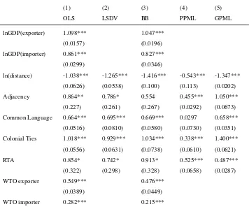
Table 2 presents the results. The interpretation of the coefficients is then as follows: the estimated coefficients present the average impact of the variables
of interest on export values fromito j, holding all other variables constant, and
setting all dummies to zero (including the regional dummies). For instance consider column (1). A 1% increase in the GDP of the exporting country leads to a 1.1%
increase in exports fromito j on average, holding all other variables constant.
Our main interest is in the distance, adjacency and world regions coefficients. First, note that the distance coefficients are more or less of the same magnitude as the cross-sectional estimates in Figure 1. However, correcting for intra-regional flows, there is a discrepancy between the OLS/LSDV/BB coefficients, and the GPML coefficient is smaller than before in absolute value.
Second, the adjacency coefficients are positive and significant at the 5% level in all settings except in the BB model. Moreover, there is quite some variation in the estimated size of the coefficient, ranging between 0.46 and 1.1. Hence for the PPML estimate of Adjacency, the interpretation is that switching the dummy from 0 to 1
increases exports fromito jwithexp(0.46)−1=58%, keeping all other variables
constant. For the GPML coefficient, this even accrues toexp(1.050)−1=186%.
Note that the adjacency dummy is mostly conditional on both countries being in the same global region, so both coefficients have to be jointly interpreted. The large variation of the estimated coefficients across methods however, shows that precise evaluation of barriers (e.g. for policy analysis) has to be interpreted with caution.
Third, there is a large amount of variation across the estimates of the region dummies. Consider for example the LSDV estimates in column (2). The negative coefficient for the Europe dummy suggests that trade between countries within
Europe isexp(−0.511)−1=40% lower than if both partners are in different trade
we control for adjacency when estimating the border effects: this captures the idea that intra-continental trade is larger for countries that also share a common border. More strikingly, estimated openness varies substantially across estimation methods in terms of size, and all regional dummies are at least insignificant at the 5% level in one specification, except that of the Pacific. Hence contrary to our findings for the distance effect, the border effect by global regions appears to be much more sensitive to the selected estimation methodology. Finally, it is interesting to note that intra-ASEAN trade is fairly low. Trade involves relatively more exports to countries outside the region, while the goal of the ASEAN union is to promote more intra-regional trade and create an internal market. Conditional on our results and estimation methods, estimation of the gravity equation indicates that this policy goal is not achieved yet.
Table 2:Borders by world regions
(1) (2) (3) (4) (5)
ln(distance) -1.038*** -1.265*** -1.416*** -0.543*** -1.347***
(0.0626) (0.0538) (0.100) (0.113) (0.0202)
Adjacency 0.864** 0.786* 0.554 0.455*** 1.050***
(0.227) (0.261) (0.267) (0.0292) (0.0673)
Common Language 0.664*** 0.695*** 0.669*** 0.0297 0.658***
(0.0516) (0.0810) (0.0580) (0.0730) (0.0351)
Colonial Ties 1.018*** 0.929*** 1.034*** 0.338*** 1.400***
(0.0556) (0.0631) (0.0738) (0.0610) (0.0621)
RTA 0.854* 0.742* 0.913* 0.525*** 0.487***
(0.322) (0.298) (0.328) (0.0658) (0.0287)
WTO exporter 0.549*** 0.476***
(0.0389) (0.0449)
(0.0316) (0.0376)
Europe -0.177 -0.511* -0.205 0.333 -0.917***
(0.214) (0.161) (0.116) (0.185) (0.0490)
North America -1.950*** -1.067*** -2.685*** -0.131 -0.451
(0.0714) (0.0794) (0.213) (0.196) (0.270)
South America 0.456* 0.491* -0.423* 0.562*** 0.518***
(0.180) (0.177) (0.135) (0.113) (0.0752)
Asia 0.191** 0.0111 0.0267 -0.0708 0.326***
(0.0481) (0.0577) (0.0451) (0.134) (0.0404)
ASEAN 0.718 -0.681* -0.890** 0.0428 -0.541***
(0.312) (0.282) (0.197) (0.179) (0.0987)
North Africa -0.259 0.679** 0.195 0.258*** -0.187
(0.251) (0.188) (0.174) (0.0338) (0.0959)
Africa 0.0996 0.207 -0.184 0.985*** 0.315***
(0.213) (0.140) (0.143) (0.138) (0.0600)
Pacific 2.537*** 1.575*** 0.549* 1.019*** 1.954***
(0.230) (0.200) (0.191) (0.159) (0.149)
Constant -17.82*** 16.49 -25.03*** 12.18*** 18.20***
(1.192) (.) (0.882) (0.936) (0.312)
Country FE No Yes No Yes Yes
adj.R2 0.671 0.735 0.678 0.794 –
BIC 1,234,183.7 1,325,030.5 1,228,427.5 6.46e+10 8,390,863.1
N 283,822 319,276 283,822 532,029 532,029
5
Robustness Checks
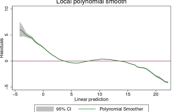
We check for several potential sources of misspecification. First, we draw the
residual versus fitted values plot for the LSDV method in Figure 2.11 Since we deal
with so many observations, traditional scatter plots are not very efficient. Instead, we propose to use a local polynomial smoother plot to represent the underlying scatters. The local polynomial has two added advantages for residual analysis: i) the polynomial smoother is an indicator for potential non-linearities or other patterns in the residuals, and ii) the 95% confidence intervals of the smoother are a nice way to depict potential heteroscedasticity: if there are irregularities in the width of the confidence intervals, this indicates non-constant variance of the error terms. We rerun the original specification of Section 4, but now for the year 2005 only,
to evade potential auto-correlation.12 There is i) a clear structure in the residuals
that resembles a third-degree polynomial and ii) potential heteroscedasticity could show up in the left tail of the distribution of the fitted values. We are confident that heteroscedasticity is not affecting our results in any major way (we also check the pattern of heteroscedasticity using PPML, giving almost identical results), and focus on the non-linear pattern of the residuals.
Second, to see where the structure comes from, we plot the residuals against each regressor. The residual plots of all regressors look fine, except the residual plot against distance uncovers the same structure as the residuals versus fitted plot. We therefore rerun the model with a polynomial approximation for distance: it might be the case that the linear specification of the distance function is just not correct, and we just assumed it following the bulk of the gravity literature. We rerun the model with a second and third order polynomial for distance, which in effect lowers the pattern in the residual plots, but completely disrupts all of the gravity
estimates. We also check if there is a non-linear patterninsideglobal regions, so
to see that the non-linearities do not come from the global sample. We see the same residual pattern recurring for each isolated subsample. We therefore prefer to keep with the mainstream of the literature and use the log-linear distance function.
11We also run the residual plots for the other estimation methods. Patterns are similar.
12We also ran the model on the pooled version and the panel version, all giving very similar results
However, the correct specification of the distance function is an interesting topic in its own.
Third, we check for potential multicollinearity between distance and the border effect, since this might also drive misspecification. We find VIF test results for all variables in the model (excluding the fixed effects) between 1 and 1.5, where VIF values of above 5 or 6 might indicate potential multicollinearity problems. We therefore also reject this potential problem.
−
5
0
5
10
Residuals
−5 0 5 10 15 20
Linear prediction
95% CI Polynomial Smoother
kernel = epanechnikov, degree = 0, bandwidth = .26, pwidth = .4 Local polynomial smooth
Notes: A local polynomial smoother represents the underlying scatter plot. The gray band indicates the 95% confidence interval, they=0 line is indicated in red.
Figure 2:Residual versus fitted plots
6
Conclusion
across estimation methods. For the border effect we distinguish between adjacency effects and regional block effects. In order to measure the border effects correctly, we simultaneously control for both border effects as well as for distance. The adjacency or contingency effect is significantly positive in all estimation methods, expect in the Baier and Bergstrand (2009) method where it is insignificant. Hence the direction of both the distance and adjacency effect appears to be in line with the literature, but their magnitudes vary substantially across estimation methods. Finally, the regional block effects are subject to a large amount of variation, both across regions and across estimation methods.
Our results point to heterogeneity across estimation methods when assessing distance and border effects in international trade. However, our results do not favor particular estimation methods, as these all have merits and shortcomings. Rather,
researchers should be aware of the impact of the selected method, thatinter alia
depends on the features of the data used in the analysis (e.g. impact of outliers). Nevertheless, we are able to provide some guidelines for future empirical research. First, the use of fixed effects is preferable. If the identification of the variable of interest is in the bilateral dimension (e.g. tariffs, non-tariff trade barriers etc.), it is suggested to use OLS with exporter and importer fixed effects. These fixed effects or dummies capture unobserved heterogeneity, including multilateral resistance terms as pointed out by e.g. Anderson and van Wincoop (2003) and Behar and Nelson (2014). If the variable of interest is in the country level dimension, identifi-cation of the variable is impossible with exporter and importer fixed effects. Then we suggest using the Baier and Bergstrand (2009) Taylor approximation approach, which approximates the trade cost variables, corrected for multilateral resistance, while leaving open the country dimension for identification.
Second, in the presence of structural zeros (such as in Helpman et al. (2008)), log-linearizing the gravity equation leads to a biased sample to perform the
esti-mation on: all zero flows drop out asln(x) is undefined for allx0. Previous
only converges under severe sample size restrictions in STATA. This is probably the reason why this procedure is not widely implemented in the empirical gravity literature.
Third, pseudo-maximum likelihood methods are linked to the gravity model through the resemblance of the first-order conditions. No other distributional assumptions on the data are required. Hence, alternative methods such as zero-inflated Poisson estimation are not at all related to the gravity model, and generate biased results.
In the end, we suggest researchers to provide a side-by-side presentation of the fixed effects (or Baier and Bergstrand 2009) and PPML approaches. Note also that we follow the theoretical gravity literature and estimate a cross-sectional gravity equation. If a researcher deems panel estimation to be appropriate, we propose estimating the model using LSDV including exporter-time and importer-time fixed effects. If the bilateral variable of interest is also time-varying, one can include country-pair fixed effects. We are aware that this dimensionality causes potential convergence problems using panel PPML in STATA (e.g. the xtpqml command).
References
Anderson, J. (1979). A Theoretical Foundation for the Gravity Equation.American Economic Review, 69(1): 106–116. URLhttp://www.jstor.org/stable/1802501.
Anderson, J., and van Wincoop, E. (2003). Gravity with Gravitas: A Solution to the Border Puzzle. American Economic Review, 93(1): 170–192. URL
https://www.aeaweb.org/articles?id=10.1257/000282803321455214.
Anderson, J., and van Wincoop, E. (2004). Trade Costs. Journal of Economic Literature, 42(3): 691–751. URLhttps://www.aeaweb.org/articles?id=10.1257/
0022051042177649.
Baier, S., and Bergstrand, J. (2009). Bonus Vetus OLS: A Simple Method for Ap-proximating International Trade-Cost Effects Using the Gravity Equation. Jour-nal of InternatioJour-nal Economics, 77(1): 77–85. URLhttp://www.sciencedirect.
com/science/article/pii/S0022199608001062.
Baltagi, B., Egger, P., and Pfaffermayr, M. (2014). Panel Data Grav-ity Models of International Trade. CESifo Working Papers 4616.
URL https://www.cesifo-group.de/de/ifoHome/publications/working-papers/
CESifoWP/CESifoWPdetails?wp_id=19106232.
Behar, A., and Nelson, B. (2014). Trade Flows, Multilateral Resistance, and Firm Heterogeneity. Review of Economics and Statistics, 96(3): 538–549. URL
https://ideas.repec.org/a/tpr/restat/v96y2014i3p538-549.html.
Behar, A., and Venables, A. (2009). Transport Costs and International Trade. In A. de Palma, R. Lindsey, E. Quinet, and R. Vickerman (Eds.),Handbook of Transport Economics, 12679. Edward Elgar Publishing.
Bergstrand, J. (1989). The Generalized Gravity Equation, Monopolistic Competi-tion, and the Factor-proportions Theory in International Trade. Review of Eco-nomics and Statistics, 71(1): 143–153.URLhttp://www.jstor.org/stable/1928061.
Bernard, A., Eaton, J., Jensen, B., and Kortum, S. (2003). Plants and Productivity in International Trade. American Economic Review, 93(4): 1268–1290. URL
https://www.aeaweb.org/articles?id=10.1257/000282803769206296.
Berthelon, M., and Freund, C. (2008). On the Conservation of Distance in In-ternational Trade. Journal of International Economics, 75(2): 310–320. URL
http://www.sciencedirect.com/science/article/pii/S0022199608000226.
Blum, B., and Goldfarb, A. (2006). Does the Internet Defy the Law of
Grav-ity? Journal of International Economics, 70(2): 384–405. URL http:
//www.sciencedirect.com/science/article/pii/S0022199606000225.
Boisso, D., and Ferrantino, M. (1993). Is the World Getting Smaller? A Gravity Export Model for the Whole Planet World? Richard Johnson Center, Working Paper 9225.
Bosquet, C., and Boulhol, H. (2010). Scale-dependence of the Negative Binomial Pseudo-Maximum Likelihood Estimator. Document de Travail 2010-39. URL
https://halshs.archives-ouvertes.fr/halshs-00535594/document.
Brun, J., Carrère, C., Guillaumont, P., and de Melo, J. (2005). Has Distance Died? Evidence from a Panel Gravity Model.The World Bank Economic Review, 19(1): 99–120. URLhttp://www.jstor.org/stable/40282208.
Coe, D., Subramanian, A., and Tamirisa, N. (2007). The Missing Globalization Puzzle: Evidence of the Declining Importance of Distance. IMF Staff Papers, 54(1): 34–58. URLhttps://www.imf.org/External/Pubs/FT/staffp/2007/01/coe. htm.
Costinot, A., and Rodríguez-Clare, A. (2014). Trade Theory with Numbers: Quantifying the Consequences of Globalization. In G. Gopinath, E. Helpman, and K. Rogoff (Eds.),Handbook of International Economics, volume 4. Elsevier.
Coughlin, C., and Novy, D. (2012). Is the International Border Effect Larger than the Domestic Border Effect? Evidence from U.S. Trade. GEP Research Paper 2009/29, University of Nottingham. URL http://papers.ssrn.com/sol3/papers.
Deardorff, A. (1995). Determinants of Bilateral Trade: Does Gravity Work in a Neoclassical World? University of Michigan Research Seminar in International Economics 382, University of Michigan Research Seminar in International Economics. URLhttps://ideas.repec.org/p/fth/michet/95-05.html.
Disdier, A., and Head, K. (2008). The Puzzling Persistence of the Distance Effect on Bilateral Trade. Review of Economics and Statistics, 90(1): 37–48. URL
http://www.mitpressjournals.org/doi/pdf/10.1162/rest.90.1.37.
Eaton, J., and Kortum, S. (2002). Technology, Geography and Trade.Econometrica, 70(5): 1741–1779. URLhttp://onlinelibrary.wiley.com/doi/10.1111/1468-0262.
00352/abstract.
Egger, P., and Staub, K. (2016). GLM Estimation of Trade Gravity Models with Fixed Effects. Empirical Economics, 50(1): 137–175. URLhttp://link.springer.
com/article/10.1007%2Fs00181-015-0935-x.
Eichengreen, B., and Irwin, D. A. (1998). The Role of History in Bilateral Trade Flows. In J. Frankel (Ed.),The Regionalization of the World Economy. National Bureau of Economic Research Project Report. University of Chicago Press.
Felbermayr, G., and Kohler, W. (2006). Exploring the Intensive and Extensive Margins of World Trade. Review of World Economics, 142(4): 642–674. URL
http://www.jstor.org/stable/40441114.
Frankel, J. (1997a). Regional Trading Blocs in the World of Economic System. Washington D.C.: Institute for International Economics.
Frankel, J. (1997b). Sterilization of Money Inflows: Difficult (Calvo) or Easy (Reisen)? Estudios de Economia, 24(2): 263–328.
Frankel, J., and Wei, S.-J. (1993). A Pacific Economic Bloc: Is There Such an Animal? FRBSF Economic, (39). URLhttps://ideas.repec.org/a/fip/fedfel/
y1993inov12n93-39.html.
Gaulier, G., and Zignago, S. (2010). BACI: International Trade Database at the Product-Level. The 1994–2007 Version. CEPII Working Paper 2010–23. URL
Gourieroux, C., Monfort, A., and Trognon, A. (1984). Pseudo Maximum Likeli-hood Methods: Applications to Poisson Models. Econometrica, 52(3): 701–720.
URLhttp://www.jstor.org/stable/1913472.
Harris, M., Kostenko, W., Matyas, M., and Timol, I. (2009). The Robustness of Estimators for Dynamic Panel Data Models to Misspecification. Singapore
Economic Review, 54(3): 399–426. URLhttp://www.worldscientific.com/doi/
abs/10.1142/S0217590809003409.
Harris, M., and Matyas, L. (2004). A Comparative Analysis of Different IV and GMM Estimators of Dynamic Panel Data Models. International Statistical Review, 72(3): 397–408.URLhttp://www.jstor.org/stable/25472630.
Head, K., and Mayer, T. (2014). Gravity Equations: Workhorse, Toolkit, and Cookbook. In G. Gopinath, E. Helpman, and K. Rogoff (Eds.), Handbook
of International Economics, volume 4, pages 131–195. Elsevier. URL http:
//www.sciencedirect.com/science/handbooks/15734404.
Helliwell, J. (1996). Do National Borders Matter for Quebec’s Trade? Canadian Journal of Economics, 29(3): 507–522. URLhttp://www.jstor.org/stable/136247.
Helliwell, J. (1997). National Borders, Trade and Migration. NBER Working Papers 6027. URLhttp://www.nber.org/papers/w6027.
Helliwell, J., and McCallum, J. (1995). National Borders Still Matter For Trade. Policy Options/Options Politique, 16(5): 44–48.
Helpman, E., Melitz, M., and Rubinstein, Y. (2008). Estimating Trade Flows: Trading Partners and Trading Volumes.Quarterly Journal of Economics, 123(2): 441–487. URLhttp://qje.oxfordjournals.org/content/123/2/441.short.
Hillberry, R., and Hummels, D. (2003). Intranational Home Bias: Some Ex-planations. Review of Economics and Statistics, 85(4): 1089–1092. URL
http://www.mitpressjournals.org/doi/pdf/10.1162/003465303772815970.
Re-view, 52(3): 527–550. URL http://www.sciencedirect.com/science/article/pii/
S0014292107000402.
Leamer, E. (1993). U.S. Manufacturing and an Emerging Mexico.North American Journal of Economics and Finance, 4(1): 51–89.
Leamer, E. (2007). A Flat World, a Level Playing Field, a Small World After All, or None of the Above? A Review of Thomas Friedman’s The World is Flat. Journal of Economic Literature, 45(1): 83–126. URLhttps://www.aeaweb.org/
articles?id=10.1257/jel.45.1.83.
Mayer, T., and Zignago, S. (2011). Notes on CEPII’s Distances Measures: The GeoDist Database. CEPII Working Paper 2011-25. URLhttp://www.cepii.fr/
CEPII/en/publications/wp/abstract.asp?NoDoc=3877.
McCallum, J. (1995). National Borders Matter: Canada-U.S. Regional Trade Patterns. American Economic Review, 85(3): 615–623. URLhttp://www.jstor.
org/stable/2118191.
Melitz, M. J. (2003). The Impact of Trade on Intra-Industry Reallocations and Aggregate Industry Productivity. Econometrica, 71(6): 1695–1725. URLhttp:
//www.jstor.org/stable/1555536.
Nitsch, V. (2000). National Borders and International Trade: Evidence from the European Union. Canadian Journal of Economics, 33(4): 1091–1105. URL
http://www.jstor.org/stable/2667393.
Novy, D. (2013). International Trade without CES: Estimating Translog
Grav-ity. Journal of International Economics, 89(2): 271–282. URL http://www.
sciencedirect.com/science/article/pii/S0022199612001584.
Obstfeld, M., and Rogoff, K. (2001). The Six Major Puzzles in International Macroeconomics: Is There a Common Cause? InNBER Macroeconomics An-nual 2000, volume 15, pages 339–412. National Bureau of Economic Research,
Robinson, P. (1987). Asymptotically Efficient Estimation in the Presence of Heteroskedasticity of Unknown Form. Econometrica, 55(4): 875–891. URL
http://www.jstor.org/stable/1911033.
Rossi-Hansberg, E. (2005). A Spatial Theory of Trade. American Economic
Review, 95(5): 1464–1491. URLhttps://www.aeaweb.org/articles?id=10.1257/
000282805775014371.
Santos Silva, J., and Tenreyro, S. (2006). The Log of Gravity. The Review of Economics and Statistics, 88(4): 641–658. URLhttp://www.mitpressjournals.
org/doi/pdf/10.1162/rest.88.4.641.
Soloaga, I., and Winters, L. A. (2001). Regionalism in the Nineties: What Effect on Trade? North American Journal of Economics and Finance, 12(1): 1–29.
URLhttp://www.sciencedirect.com/science/article/pii/S1062940801000420.
Tinbergen, J. (1962).Shaping the World Economy; Suggestions for an International
Economic Policy. Twentieth Century Fund, New York.
Wei, S.-J. (1996). Intra-National versus International Trade: How Stubborn Are Nations in Global Integration? NBER Working Papers 5531. URLhttp://www.
nber.org/papers/w5531.
White, H. (1980). A Heteroskedasticity-Consistent Covariance Matrix Estimator and a Direct Test for Heteroskedasticity. Econometrica, 48(4): 817–838. URL
http://www.jstor.org/stable/1912934.
Please note:
You are most sincerely encouraged to participate in the open assessment of this article. You can do so by either recommending the article or by posting your comments.
Please go to:
http://dx.doi.org/10.5018/economics-ejournal.ja.2016-18
The Editor