www.elsevier.nl / locate / econbase
Labor and capital income taxation, fiscal competition,
and the distribution of wealth
*
Clemens Fuest , Bernd Huber
¨ University of Munich, Staatswirtschaftliches Institut, Ludwigstr. 28, VG., III, D-80539 Munchen,
Germany
Received 30 July 1998; received in revised form 30 November 1998; accepted 1 December 1998
Abstract
This paper studies optimum income taxation in a small open economy where households differ with respect to their endowments with wealth. The government raises taxes on income from labor and wealth and a source tax on capital used in domestic production. To avoid taxes, households may, at some cost, shift capital to labor income and vice versa. The government can only observe income after shifting has taken place. It turns out that the optimal source tax on capital is negative. The optimal income tax is characterized by a positive marginal tax rate for the wealthy households, which is equal for labor income and income from wealth. For the poor households, the marginal tax rate on capital income is higher than that on labor income. We also study international tax coordination and show that a reduction in the source subsidy on capital raises welfare. 2001 Elsevier Science B.V. All rights reserved.
Keywords: Optimum income taxation; Wealth taxation; Fiscal competition JEL classification: H21; H24; F 21
1. Introduction
The standard optimum income tax model (Mirrlees, 1971; Stiglitz, 1982, 1987) analyzes the optimal design of redistributive policies between agents who differ in
*Corresponding author. Tel.:149-89-2180-6339; fax:149-89-2180-3128. E-mail address: [email protected] (C. Fuest).
1
their abilities and, thus, the wage rates they can earn in the labor market. In this model, informational constraints prevent that a first-best optimum can be attained. The nature of the resulting second-best problem in this framework has been extensively studied in numerous contributions which have immensely added to our
2
understanding of second-best redistributive policies.
On the other hand, this approach has its limitations as it only deals with redistribution between wage earners with differing abilities. Empirically, in-dividuals differ not only in their abilities (wages), but also – perhaps even more importantly – in their levels of wealth. It is well known that, in most countries, wealth is rather unevenly distributed such that a small group of households holds a disproportionately large share of aggregate wealth. The wealth distribution also affects the distribution of income as high incomes are often incomes accruing from wealth.
It is important to note that the standard optimum income tax model can, in principle, account for the role of wealth if differences in individual wealth can be explained by the different abilities of individuals. One may argue that high ability (high income) individuals accumulate more wealth over their life cycle than low ability ones. In this case, the Stiglitz–Mirrlees model again represents the appropriate framework for tax policy analysis. By adding an intertemporal savings choice to this model, one can then study the optimal tax treatment of capital or, more generally, wealth. It turns out that, under rather mild assumptions, capital should not be taxed (see Atkinson and Stiglitz, 1976; Stiglitz, 1982, 1987).
One problem with this argument is that different abilities are the only exogenous source of heterogeneity between individuals. But one can plausibly argue that heterogeneity may also arise from exogenous endowments with goods and factors,
3
i.e. wealth, which vary across individuals. Introducing a second dimension of diversity, however, severely complicates the optimal tax problem since one then
4
has to solve a two-dimensional adverse selection problem. In this paper, we therefore concentrate on a simpler case where exogenous variations in endow-ments (wealth) are the sole source of heterogeneity.
We consider a model with two types of agents. Both earn the same wage rate but their exogenous endowments with capital differ. The government in this model
1
Nonetheless, the government’s problem is often modelled as a pareto-optimizing one (see Stiglitz, 1982).
2
See Tuomala (1990) for a survey and Boadway (1995) for a wide-ranging discussion of potential applications of this approach.
3
One may criticize this on the ground that these endowments are not truly exogenous and reflect past savings choices. Treating them as exogenous is then misleading and reflects a time inconsistency problem along the lines of Fischer (1980). One may first note that this argument is to some extent a philosophical one whether there truly exists something like exogenous endowments. Furthermore, it is also clear that a similar argument can be made concerning abilities which are also not truly exogenous as they may reflect educational choices of families perhaps in the very distant past.
4
wishes to redistribute from the wealthy households to the ‘‘poor’’ households and can impose (non-linear) taxes on labor income and capital income. But the government also faces informational constraints restricting the scope of redistribu-tive policies. Individual wealth and labor supply cannot be directly observed. The government also cannot directly infer a person’s true type by observing his / her labor and capital income because taxpayers may shift labor to capital income, and vice versa. In our model, income shifting does not lead to outright tax evasion but it means that, at some cost, taxpayers may transform capital income into labor
5
income, and vice versa. As a consequence, a self-selection constraint for the wealthy individual which restricts redistributive policies has to be taken into account.
A second feature which is highly relevant for the taxation of wealth is the phenomenon of fiscal competition. We therefore model the country as a small open economy with perfect capital mobility. In this context, the capital income tax imposed on domestic households represents a residence-based tax on capital, albeit an imperfect one due to the opportunity of income shifting. In addition to the taxation of domestic households’ income, the government can levy a source tax on capital employed in domestic production.
We first characterize the optimal tax policy in this small country. If there are no source-based capital taxes, the marginal tax rate on labor income for wealthy individuals is zero. This result essentially parallels the no distortion at the top result of the standard optimum income tax framework. It is interesting to note that this key property of the Mirrlees–Stiglitz approach also holds in our model where differences in capital endowments are the source of heterogeneity between individuals. If the government levies a source tax on capital, a somewhat different picture emerges. It now turns out that the optimal source tax on capital is negative. In this case, the marginal labor income tax rate on wealthy individuals is strictly positive. The economic purpose of this positive tax is to correct a labor supply
6
distortion induced by the (optimally chosen) source tax on capital. Furthermore, we can show that marginal tax rates on capital and labor income of wealthy individuals are equalized.
We also study whether national tax policies lead to globally efficient outcomes. Our main result is here that uncoordinated fiscal policies are characterized by inefficiently low source taxes on capital. It is interesting to contrast these results with other findings in the fiscal competition literature. In an important contribu-tion, Bucovetsky and Wilson (1991) demonstrate in a representative agent model that uncoordinated fiscal equilibria are efficient if a residence-based tax on capital
5
That precisely this type of income shifting limits the possibility of taxing different types of income at different rates is discussed in Gordon and MacKie-Mason (1995) and Gordon (1998).
6
income is available. Further research has made clear that this result deserves some qualification. For example, Huizinga and Nielsen (1997) have shown that global efficiency with residence based taxation critically depends on the assumption of domestic ownership of firms. Our findings point into a similar direction. In our model, such a residence-based tax is available, although it is subject to income shifting problems. Yet, national tax policies are not globally efficient.
The paper is organized as follows: In Section 2, we introduce the model. Optimal tax policy for an individual country is analyzed in Sections 3 and 4. In Section 5, we discuss the efficiency properties of national fiscal policies and the potential for welfare-enhancing tax coordination. Conclusions are given in Section 6.
2. The model
2.1. Households
The model we use incorporates three features: the role of the distribution of wealth, the tax treatment of labor income and income from wealth, and the effects of fiscal competition on tax policy. As was explained, this model differs in several respects from the standard optimal income tax framework of Stiglitz (1982). We will therefore take some care to describe the key building blocks of the model.
We consider a small open economy with two types of individuals denoted by 1 and 2, respectively. Individuals have the same strictly quasi-concave utility function U C ,Ls i id where C is consumption of person i and L is his / her labori i
supply (i51, 2). Individuals have two sources of income, labor income and capital income. Person i’s (pre-tax) income from labor supply amounts to wL . In contrasti
to the standard optimum income tax model, we assume that both types of individuals earn the same wage rate. This assumption serves to focus on differences in individual wealth which we discuss below. One may also note that labor supply refers to employment at domestic firms, i.e. we assume that labor is internationally immobile.
To capture the role of the wealth distribution, we assume that persons have different endowments E with capital. As a matter of convention, we consider thei
case E2.E , i.e. person 2 is wealthier than person 1. As was mentioned above,1
the levels of wealth, i.e. the endowments E , are exogenously given in our analysis.i
We thus abstract from intertemporal savings decisions in our model. The main reason is that even the simple static environment we consider gives rise to a complex optimal tax problem which would be further complicated by introducing
7
an intertemporal dimension into the analysis.
7
Capital is internationally mobile in this model. Person i earns the amount of (pre-tax) capital income rE where r denotes the world interest rate which isi
exogenously given for the country. Notice that r is the return on capital net of source (withholding) taxes.
The government cannot directly observe a person’s labor supply or wealth. But individuals have to report their labor income and capital income (income from wealth) for tax purposes. Yet, this does not allow the government to directly infer a person’s true labor supply and wealth as individuals have the possibility to shift labor to capital income and vice versa. In the following, the income after potential income shifting has taken place is referred to as reported income. We denote person i’s reported capital income by rK such that r(Ei i2K ) is shifted to labori
income. We allow for income shifting into both directions Ks i#E and Ki i$E .id
Notice that income shifting in this context is a purely domestic problem while
8
there are no problems of international tax evasion. Thus, the government does not face any specific difficulties to tax capital income earned abroad. Capital income taxation therefore amounts to a residence based tax on worldwide capital income. We focus instead on the problem that total capital income from domestic and foreign sources may be shifted to labor income and taxed accordingly.
Income shifting involves some costs which are given by z r Es s i2Kiddwhere z(?)
9
is a non-negative and convex function with z 0s d50 and z9s d0 50 and z9 ` ,s d 1. The idea of this cost function is to capture in a very simple way the idea that income shifting is costly for an individual.
Reported labor income Y of person i is given by Yi i5wLi1r Es i2Kid2
10
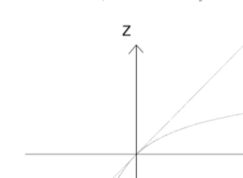
z r Es s i2K .idd For further purposes, define the function Z r Es s i2Kidd5r Es i2 Kid2z r Es s i2Kidd which is monotone and concave with Z(0)50 and Z9s d0 51. Z(.) gives shifted capital income net of shifting costs and is illustrated in Fig. 1. If rEi.rK , the person shifts capital to labor income. For a given labor supply,i
reported labor income then increases by Z. The difference between the (dotted) unit line in Fig. 1 and the Z(.) function reflects that income shifting is costly. This also applies if labor income is shifted to capital income. If rEi,rK , taxable labori
income is reduced by 2Z while capital income is increased by r(Ki2E ).i
We have chosen this formulation of income shifting to introduce in a simple way some restraint on feasible capital income taxation. As explained below, the government in this model wishes to redistribute from wealthy households of type 2 to ‘‘poor’’ households of type 1. This could in principle be achieved by imposing a
8
An optimum income tax model with international tax evasion is discussed in Huber (1997). 9
A similar type of cost function is employed in Boadway et al. (1994). One difference is that their model deals with problems of tax evasion while, in our model, the agents are only allowed to shift income from one type of income to the other. We do not assume strict convexity as in the paper of these authors to allow for the case that income shifting costs are zero.
10
Fig. 1. Capital income net of shifting costs (Z ) as a function of shifted income.
high tax on capital income which is borne to a large extent by the wealthy individuals. But, if income shifting is possible, the government’s ability to increase capital income taxes is restricted because individuals have an incentive to shift asset income to labor income.
The government in this model observes labor and capital income after income shifting has taken place, i.e. Y and rK , of the two persons, i51, 2, and imposes ai i general non-linear tax schedule T(Y , rK ) based on this information. Consumptioni i
of person i is thus given by
Ci5Yi1rKi2T Y , rKs i id (1)
where
Yi5wLi1Z r Es s i2Kidd (2)
Using (2), one can express the utility of household i as a function of the variables C , Y and rK which the government can actually observe. Formally, this definesi i i
i
the function Vs d? with
Yi2Zi
i
S
]]
D
V C , Y , K , r, ws i i i d5U C ,i w (3)
11
where Zi5Z r Es s i2K .idd
11
For further use, we note that
where VC denotes the partial derivative with respect to C and so on.i
Finally, we briefly analyze household i’s problem which is to maximise (3)
12
subject to (1). First-order conditions are
i i i
where T , TY K denote the marginal tax rates on reported labor and capital income individual i faces. Note that (4) is a standard marginal condition for consumption– labor choice. Combining (4) and (5), one obtains
i
12TK
]]i 5Z9i (6)
12TY
i i
which reflects the impact of taxation on income shifting. If TK.T , theY
household will shift capital to labor income (Ei.K and Z(i ?).0) to benefit from
i i
the lower marginal tax rate on labor income. The opposite applies if TK,T . NoY
income shifting occurs if the marginal tax rates on capital and labor income are equal.
2.2. Production
Output is produced according to a constant-returns-to-scale production function F N Ls 1 11N L , K2 2 d where K denotes the capital stock. Since both types are assumed to earn the same wage w, total labor supply N L1 11N L2 2 enters the production function. (Perfect) international capital mobility implies that the small country faces an infinitely elastic supply of capital at the world interest rate r. The existence of a world capital market also means that the capital stock employed in
12
domestic production (domestic investment) bears no direct relation to the wealth of households N E1 11N E (domestic savings).2 2
The government levies a source tax on capital K at rate tk. The marginal productivity condition for capital is then given by
f9s dk 5r1tk (7)
where k5K / N Ls 1 11N L2 2d denotes capital per unit of labor. f(k) is the corre-sponding per capita production function. This condition can be solved for k rs 1tkd
with k9 51 /f0 ,0. Using the fact that w5f ks d2sr1tkdk, one obtains the factor– price frontier
w5w rs 1tkd (8)
with w9 5 2k,0.
Finally, one can now state the country’s aggregate resource constraint which is
N C1 11N C2 2#( f(k)2rk) N Ls 1 11N L2 2d1rN E1 11rN E2 22N z1 12N z2 2
(9)
where we have assumed, since we are mainly interested in redistributive tax policy, that exogenous government spending on goods and services is zero.
3. The government’s problem
In this section, we now turn to the government’s optimal tax problem. We proceed in two steps. We will first discuss the structure of the national planner’s optimal tax problem in some detail. In the following section, we then derive the optimal tax policy.
In what follows, we assume that the government maximizes a utilitarian social welfare function. This implies that the government wishes to redistribute from wealthy households of type 2 to households of type 1. The planner’s problem is set up as follows: since the non-linear tax schedule T(Y , K ) allows the government toi i
indirectly control C , Y and K , we pose the problem such that the planner directlyi i i
sets these variables, and we then discuss the tax policy which is required to achieve this outcome.
As a benchmark, consider first the full information case, where the government
13
can observe each individual’s labor supply L and endowment E . The problem ofi i
1 2
the government is then to maximize social welfare N V (?1 )1N V (2 ?) subject to the aggregate resource constraint (9). The solution to this problem yields a first-best optimum. Marginal utilities of the two types of households are equalized
13
1 2 i i i i V 5V . The first-best is also characterized by T 5T 50 such that V 5V
s
C Cd
Y K C Yand Zi50. To implement the first-best, lump-sum taxes conditioned on E are seti
14
which achieve an optimal redistribution from type 2 to type 1 households. In the presence of informational constraints, the first-best optimum can no longer be attained because it is not incentive-compatible. If the government can only observe Y and rK , person 2 will mimic person 1 if the government tries toi i
15
implement the first-best.
Due to these informational constraints, the government has to solve a second-best problem. In this setting, redistributive policies are limited by the self-selection constraint which precludes that person i, i51, 2, can gain by mimicking person j, j±i. Denote a mimicker by a bar. If person 2 mimicks person 1, this yields
] mimicker, person 2 has to report the same labor income as person 1 (Y ), the labor1
supply of person 2 will be less than that of person 1. The opposite applies if person 1 mimics person 2. Thus, a mimicker would choose his labor supply so that, given
16
the amount of shifted income, the observable variables match the required levels. The self-selection constraint for a person of type i requires
]
i i
V C , Y , K , r, w, Es d$V C , Y , K , r, w, E
s
d
i51, 2, j±1. (10)i i i i j j j i
In the standard optimum income tax model with differing abilities, the well-known monotonicity property rules out that the self-selection constraints of both persons
17
bind. In our model, the appendix derives sufficient conditions which ensure for fairly general utility functions that an analoguous property holds, implying that only the self-selection constraint for the wealthy individual binds.
14 i 2
Denoting optimal lump-sum taxes by T , one obtains T 5r Es 22E1dsN / N1s 11N2dd.0 and
1 2
T 5 2sN /N T2 1d ,0. 15
This can be seen as follows. Using the tax formula in footnote 12, it is straightforward to check that a first-best optimum implies C15C25C and Y15Y25Y. If person 2 (the high-wealth individual) reveals his true type, utility is thus given by U(C, Y /w). If person 2 mimics person 1, person 2 again achieves C as level of consumption. Person 2 then reports the same income and pays the same amount of taxes as person 1 in the first-best. Mimicking also implies that the amount r(E22K ) of capital1 income is shifted to labor income. Total utility of a mimicker is thus given by U(C, (Y2Z(r (E22K )) /w)). But since Z1 .0, this implies that a mimicking strategy strictly dominates truth-telling in a first-best optimum. This reflects that the (wealthy) mimicker gains by supplying less labor while consumption remains constant, as explained in the next paragraph in the text.
16
We owe this explanation to a referee. 17
4. Optimal tax policy
In this section, we now derive the government’s optimal tax policy. As was discussed in the last section, the problem of the government in this country is to
1 2
maximize social welfare N V (1 ?)1N V (2 ?) subject to (i) the self-selection constraint of person 2 and (ii) the aggregate resource constraint. The Lagrangean [( ) of this problem may be written as:
1 2
wherel, m are Lagrangean multipliers. Notice also that w and k are functions of r1tk.
The first-order condition fortk is cumbersome.
Using (11a)–(11f), one can simplify this expression and obtains after some manipulation
]2 ]
lV ZY
s
12Z2d
5mtksN1a 11 N2a2dk9 (12b) Assuming that the solution to (11) and (12) is a global optimum, we can now work out the implications of these conditions for optimal tax policy.4.1. No source-based capital tax (t 50)k
It is helpful to begin with the simple benchmark case wheret 5k 0. The country will always chooset 5k 0 if the elasticity of substitution between labor and capital is infinite k9 5 2 `s d. An example is a linear technology under which the marginal product of all factors is constant. Optimal policy is then described by (11) with
2 2
t 5k 0. Eqs. (11d)–(11f) for t 5k 0 immediately yield that Ty5TK50, i.e. the marginal tax rate on the wealthy individual is zero. The equalization of marginal tax rates on labor and capital income also implies that individual 2 has no incentive to shift income. This is a variant of the well-known no distortion at the top-result and closely resembles the results from the standard optimum income tax model. It is interesting to note these parallels, since the source of individual heterogeneity in our model lies in different capital endowments while the standard model refers to differences in individual productivities. Along these lines, one can also show that the marginal tax rate on labor income for individual 1 is positive.
1 1
Eq. (11c) yields that, at the optimum, TY diverts from T , i.e. there will be someK
income shifting by individual 1. In this context, socially costly income shifting is used as an instrument to affect mimicking behavior in a way that will be explained further below.
4.2. Optimal tax policy with j ±0
k
We now discuss optimal tax policy when the source tax can be imposed. A source tax can be levied in an economically meaningful way if the elasticity of substitution is finite such that k9is finite. In this case, one obtains the result that the optimal source tax is negative. This is easily verified in (12b) by noting that
]
k9 ,0 and Z2.Z . We may thus state1
Proposition 1. If the elasticity of substitution is finite, the optimal tax policy
imposes a negative source tax on capital (a subsidy).
18
2kdt .k 0. For a given labor supply L (L ) person 1(2) will earn an additional1 2
2kL d1 t 2ks kL d2 tkd. Government outlays for this subsidy amount to 2sN L1 11 N L kd2 2d tk. Thus, an additional lump sum tax 2L kd1 tksL kd2 tkdon person 1(2) will leave utility of both types of households unchanged and will ensure that this subsidy can be paid for. The key point is that this policy makes a mimicker worse
]
off. Since E2.E , his labor supply L is lower than L . The mimicker therefore1 2 1
gains less from the higher wage than he has to pay as additional tax, and his utility declines. This amounts to a weakening of the self-selection constraint which improves welfare. In the optimum described by (12b), the marginal welfare gain from relaxing the self-selection constraint has to be weighed against the resource cost of the subsidy in terms of its distortionary impact on factor input decisions. Consider first the emerging tax structure for the wealthy individual. Eqs. (11d) and (11e) now reveal that the marginal tax rate on labor income for individual 2 is
2
positive
s
TY.0 . Furthermore, one obtains that, for persons of type 2, thed
marginal tax rates on capital income and labor income are equalized. We thus obtainProposition 2. The optimal tax policy imposes (i ) a strictly positive marginal tax
rate on labor and capital income of wealthy (type 2) individuals which is (ii )
equal for the two types of income.
It is interesting to contrast this result with the existing optimum income tax literature. First, it is the positive marginal tax rate on wealthy (or, in other words, high income) individuals which is noteworthy. The standard model predicts that
19
the marginal tax rate on high income individuals is zero or even negative. The intuition for this result is the following. As explained above, the optimal policy imposes a source subsidy on capital. This subsidy has the function to weaken the self-selection constraint. However, since it raises the wage rate, it has the side effect to raise labor supply beyond the socially optimal level. The positive marginal income tax corrects for this distortion. Thus, this tax achieves a corrected
20
no distortion at the top outcome.
Secondly, we observe that it is not optimal to have income shifting by the wealthy individuals. The optimum income tax therefore sets the same marginal tax rate for labor and capital income of wealthy individuals. This can again be seen as a variant of the standard no distortion at the top result.
18
Here, one may note that a wage subsidy paid to firms would have a similar effect as the capital subsidy. However, as the following analysis concentrates on the issue of tax competition and the interaction of the source tax (or subsidy) on capital and the residence based income tax, we restrict our attention to the capital subsidy.
19
See Stiglitz (1987). 20
For the poor (type 1) individuals, some income shifting will occur in the optimum. To see this, note that Eq. (11b) implies
]
Substituting into (11c) yields, after some rearrangements:
]2 ]
Proposition 3. For the poor (type 1) individuals, the optimal marginal tax rate on
capital income is higher than the marginal tax rate on labor income.
1 1
The intuition for this result is the following. The result TK.TY implies that poor individuals will shift some capital income to labor income. The reason for this distortion is that it weakens the self-selection constraint. To see this, consider a situation where the two marginal tax rates are equal. In this case, a poor household will undertake no income shifting while a wealthy mimicker would by definition shift part of his capital income to labor income. Assume now that the government slightly raises the marginal tax rate on capital income above that on labor income. The mimicker would depart from a situation where he already undertakes some income shifting and therefore faces a strictly positive marginal cost of shifting further capital income to labor income. The increase in the marginal capital income tax rate thus imposes a cost on a mimicker while a wealthy household revealing his true type is not affected, which means that the self-selection constraint is relaxed. Of course, the higher marginal capital income tax rate also induces some income shifting by the poor household, but, since he departs from a situation without income shifting, the cost of doing so is small since the marginal cost of income shifting for this household is zero (z9(0)50). Proposition 3 shows that it is welfare-enhancing to induce a small amount of income shifting by poor individuals in exchange for making mimicking less
21
attractive.
Finally, one may ask whether the marginal income tax rates for the poor individual are generally positive or negative. Here, the most general result that can be derived holds for additively separable utility functions. Using (11a) and (11b), we obtain
Suppose that the utility function takes the form
Proposition 4. If preferences are additively separable between consumption and
leisure, the marginal tax rates on labor and capital income of the poor individuals
are both positive.
The intuition for the result in Proposition 4 is analogous to the explanation of the positive income tax rate of rich individuals.
5. Global efficiency
So far we have discussed optimal tax policy from an individual small country’s point of view. In this section, we ask whether policies where each country maximizes national welfare are globally efficient. This is, of course, a key issue in the fiscal competition literature. To study this question in our model, we assume
22
that there are M identical countries of the type described above. Each of these countries chooses its optimal tax policy according to the analysis in the previous section. In this framework, one now has to take into account an equilibrium condition for the global capital market which equates demand to supply of capital of the M countries. Concentrating on a symmetric equilibrium, the condition for capital market equilibrium requires N E1 11N E2 25K such that each of the identical countries demand for capital K must, in equilibrium, equal each country’s endowment. This equilibrium condition can be written as
k ]
N E1 11N E2 25wf sN Y1 12Z1d1N Y2s 22Z2dg (13)
22
The uncoordinated equilibrium that emerges if each country maximizes national social welfare is completely described by Eqs. (11)–(13). These conditions determine the equilibrium values of C , Y , K ,i i i tk and r.
We will now analyze whether this uncoordinated equilibrium is efficient. Intuition suggests that the source tax on capital may offer some room for a welfare improving coordination of tax policies. As explained above, an individual country levies a negative source tax on capital. But, for the M countries as a whole, it is clear that, in a symmetric equilibrium, the capital stock is fixed at N E1 11N E . A2 2
coordinated reduction in this source subsidy would therefore leave each country’s capital stock unaffected. It is then natural to ask whether such a coordinated tax change may increase welfare. In what follows we will therefore analyze the effects of such a coordinated increase in the source tax on capital.
We begin with the description of the tax coordination arrangement. Starting from the uncoordinated equilibrium, the M countries agree on a joint reduction of the existing source subsidy by dt .k 0. In addition, we assume that countries also agree to leave Y , Z , ii i 51, 2, unchanged. We make this assumption to determine the resulting change in the equilibrium interest rate in a particularly simple way. Namely, if Y , Z are kept constant, the labor supply is unchanged in this taxi i
coordination arrangement. Since the capital stock also does not change under a symmetric equilibrium, Eq. (13) then implies that the equilibrium interest rate will decrease by dr5 2dtk. As d rs 1t 5kd 0 it also follows that the wage rate is not affected by this coordinated policy change.
According to this tax coordination scheme, each country sets dY15dY25dZ15 dZ 50. Since Z 50 as E 5K , this implies dK 50. For person 1 where Z±0,
2 2 2 2 2
one obtains
1 ]
dK15r sE12K dr1d (14)
For a symmetric equilibrium, the effects of this tax coordination arrangement are given by the change in the Lagrangean[(?) in a representative country. The total differential of [ yields
] ]2
d[ 5lV dZY 21msN E1 11N E d2 2d t 1 mN K dr1 1 1mN K dr2 2 1mN rdK1 1
(15)
] ] 23
where dZ25Z2fsE22K dr2d 2rdK .1g Using (14) and dr5 2dtk, this expression becomes
]2
d[ 5 2lV EYs 22E d1d t .k 0 (16)
Thus, a coordinated increase in the source tax will unambiguously increase
23
welfare. This result is again best explained in terms of mimicking behavior. The higher source tax raises k(N E1 11N E )d2 2 tk as additional tax revenue. This allows the government to compensate type 1 (type 2) households for the decline in their
24
capital income which amounts to E dr(E dr) via a lump-sum transfer.1 2 While this leaves the utility of both households unchanged the utility of a mimicker falls. While his capital income declines by E dr he only receives E dr as compensation.2 1
The utility loss of the mimicker relaxes the self-selection constraint and, thus,
25
raises social welfare. This result is summarized by
Proposition 5. Starting from the uncoordinated equilibrium, a marginal increase
in the source tax on capital is welfare-improving.
It is interesting to contrast this finding with the results in Bucovetsky and Wilson (1991). In their (representative agent) model, these authors show that uncoordinated fiscal equilibria are efficient if countries can impose a based tax on capital income. In our model, countries can levy such a residence-based tax albeit an imperfect one due to income shifting problems. It turns out that although an imperfect residence bases tax is available the uncoordinated equilib-rium is still inefficient.
6. Concluding remarks
In this paper, we have studied an open economy optimum income tax model where agents differ with respect to endowed wealth. While this model yields some insights into the role of capital and labor income taxation in this situation, the underlying framework is a very simple one. Two important aspects we have neglected are the following: first, we have left out any differences in individual abilities which are the key elements of the standard optimum income tax model. Second, we have neglected any effects of capital taxes on intertemporal savings and investment decisions. It is clear that an overall assessment of the capital tax cannot be made without taking these intertemporal aspects into account. We hope to extend the analysis into this direction in future research.
24
In addition, the government has to undertake a revenue-neutral adjustment of person 1’s reported capital income K to keep Z constant.1 1
25
Acknowledgements
The authors would like to thank Helmuth Cremer, Ulrich Hange, Toshihiro Ihori, Søren Bo Nielsen, Achim Wambach, the participants of the International
` Seminar on Public Economics (ISPE) on Bequest and Wealth Taxation, Liege, 18–20 May 1998, and two anonymous referees for very useful comments and suggestions. The usual disclaimer applies.
Appendix A
In this appendix, we further analyze the self-selection constraints underlying the optimal tax problem in Section 4. Formally, the optimal tax problem is to maximize social welfare subject to the self-selection constraints of both in-dividuals, 1 and 2, and the aggregate resource constraint. Three types of solution can emerge for this optimization problem. The optimum is either characterized by
(i) a pooling equilibrium (C15C , Y2 15Y , K2 15K ) where both self-selection2
constraints are binding by definition
(ii) a separating equilibrium where both self-selection constraints are binding (iii) a separating equilibrium where only one self-selection constraint is binding.
In Section 4, we analyze case (iii). The purpose of this appendix is to demonstrate that it is indeed valid to concentrate on case (iii). While we do not provide a full general analysis, we will derive a sufficient condition which allows us to rule out cases (i) and (ii) such that case (iii) emerges in the optimum.
In what follows, we assume throughout that preferences are additively separ-able. More precisely, the utility function takes the form
U h Cs s d2g Ls dd (A.1)
where U9 .0, U0 ,0, h9 .0, h0 ,0, g9 .0, g0 $0. For further analysis, we define
g Ls d5L1ef L ,s d (A.2)
wheree $0, and f9 .0, f0 .0.
A.1. The case with e 50
Ife 50, the self-selection constraints (10) of individuals 1 and 2 can be written as
X11Z r Es s 12K1dd$X21Z r Es s 12K2dd (A.3)
X21Z r Es s 22K2dd$X11Z r Es s 22K1dd (A.4)
where Xi5Ci2Y . X can be seen as a composite good in the case of a lineari i
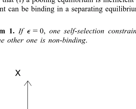
disutility of work. For simplicity, we have normalized the wage rate w to unity. For the utility function U Xs 1Z r Es s 2Kddd, one can derive indifference curves in X, rK space as in Fig. 2.
Indifference curves are upward-sloping with slope S X,K,Es d5Z9and are strictly convex. Convexity follows since≠Z9/≠(rK )5z0 .0. Fig. 2 reveals that indiffer-ence curves of type 1 (poor) individuals are steeper than those of type 2 individuals. This is so since≠S /≠E5 ≠Z9/≠E5 2z0r,0. Thus, it turns out that a standard monotonicity property holds ife 50. Using this, it is now straightforward to show that (i) a pooling equilibrium is inefficient and (ii) only one self-selection constraint can be binding in a separating equilibrium. This can be summarized by
Theorem 1. If e 50, one self-selection constraint is binding, at the optimum,
while the other one is non-binding.
A.2. The case with e .0
Suppose without loss of generality that, fore 50, the self-selection constraint of type 2 is binding (this is also the case analyzed in the main text). Fore 50, the self-selection constraints of the two individuals may be written as
] ]
X11Z11ef Ls d1 .X21Z11ef L
s d
1 (A.5)] ]
X21Z21ef Ls d2 5X11Z21ef L
s d
2 (A.6)]
where L denotes labor supply of type i if he / she mimics type j. While (A.5) andi
(A.6) hold for e 50, there also exist values of e .0 such that, at an optimum, (A–1.5) continues to hold as a strict inequality while (A.6) holds as equality. This is so sincee can be chosen arbitrarily close to zero. This gives
Theorem 2. There existvalues ofe .0 such that only one of the two self-selection
constraints is binding, at the optimum.
A.3. Discussion of results
Summing up, we have shown that there exist additively separable utility functions where only one self-selection constraint is binding, at the optimum. Using this (sufficient) condition, we can, therefore, conclude that the analysis in the main text applies at least to this type of preferences.
Appendix B
In this appendix, we would like to sketch an alternative approach for the derivation of our results. While the analysis in the main text employs a technique familiar from Stiglitz (1982), the following approach is different but allows to
26
derive the results in a somewhat simpler way. Define the amount of capital income that individual i shifts to labor income as Pi;Ei2K . Denoting thei
variables chosen by a type 2 individual mimicking type 1 by a bar, we have ]
P5P11E22E1
] ]
and, since the declared labor income of the mimicker, wL1Z(rP), would have to equal that of type 1,wL11Z(rP ),1
] Z(rP )2Z(rP)
] 1
]]]]] L5L11
w
26
The self-selection constraint for type 2 individuals can then be written as
U(wL21rE22z(rP )2 2T ,L )2 2 $U(wL11rE12z(rP )1 2T ,L1 1
] Z(rP )1 2Z(rP) ]]]]]
1 ) (B.1)
w
If this self-selection constraint is binding, i.e. (B.1) holds with an equality, the result that P 50 (Proposition 2, part ii) directly follows since, if P ±0, the
2 2
government can always raise the utility of (truth-telling) type 2 individuals and relax the self-selection constraint by setting P to zero. This would neither affect2
the government budget constraint nor make type 1 individuals worse off. Setting P250, the optimal tax problem can now be solved by maximizing
N U(wL1 11rE12z(rP )1 2T ,L )1 1 1N U(wL2 21rE22T ,L )2 2 (B.2)
over L ,P ,T ,L and T , subject to the binding self-selection constraint (B.1) and1 1 1 2 2
the government budget constraint
N T1 11N T2 21(N L1 11N L )k2 2 t $0. (B.3)
The first-order conditions can then be rearranged to yield the results in Proposi-tions 1–4.
References
Armstrong, M., 1996. Multiproduct nonlinear pricing. Econometrica 64, 51–76.
Atkinson, A.B., Stiglitz, J.E., 1976. The design of tax structure: Direct versus indirect taxation. Journal of Public Economics 6, 55–75.
Boadway, R., 1995. The role of second-best theory in public economics. EPRU Discussion Paper No. 6.
Boadway, R., Marchand, M., Pestieau, P., 1994. Towards a theory of the direct–indirect tax mix. Journal of Public Economics 55, 71–88.
Bucovetsky, S., Wilson, J.D., 1991. Tax competition with two tax instruments. Regional Science and Urban Economics 21, 333–350.
Fischer, S., 1980. Dynamic inconsistency, cooperation and the benevolent dissembling government. Journal of Economic Dynamics and Control 2, 93–107.
Gordon, R.H., MacKie-Mason, J.K., 1995. Why is there corporate taxation in a small open economy? The role of transfer pricing and income shifting. In: Feldstein, M.S., Hines, J.R. (Eds.), The effects of taxation on multinational corporations. University of Chicago Press, Chicago, pp. 67–91. Gordon, R.H., 1998. Can high personal taxes encourage entrepreneurial activity? IMF Staff Papers 45,
49–80.
Huber, B., 1997. Tax competition and tax coordination in an optimum income tax model. EPRU Discussion Paper No. 25, forthcoming in Journal of Public Economics.
Huizinga, H., Nielsen, S.B., 1997. Capital income and profit taxation with foreign ownership of firms. Journal of International Economics 42, 149–165.
Nava, M., Schroyen, F., Marchand, M., 1996. Optimal fiscal and public expenditure policy in a two-class economy. Journal of Public Economics 61, 119–137.
Rochet, J.C., 1995. Ironing, sweeping and multidimensional screening. Working paper.
Stiglitz, J.E., 1982. Self-selection and pareto efficient taxation. Journal of Public Economics 17, 213–240.
Stiglitz, J.E., 1987. Pareto efficient and optimal taxation and the new new welfare economics. In: Auerbach, A.J., Feldstein, M.S. (Eds.), Handbook of Public Economics, Vol. 2. Elsevier, North-Holland, pp. 991–1042.