www.elsevier.com/locate/dsw
An interior point method for solving systems of linear equations and
inequalities
Markku Kallio
∗, Seppo Salo
Helsinki School of Economics, Runeberginkatu 14-16, Helsinki 00100, Finland
Received 1 March 1999; received in revised form 1 March 2000
Abstract
A simple interior point method is proposed for solving a system of linear equations subject to nonnegativity constraints. The direction of update is dened by projection of the current solution on a linear manifold dened by the equations. Infeasibility is discussed and extension for free and bounded variables is presented. As an application, we consider linear programming problems and a comparison with a state-of-the-art primal–dual infeasible interior point code is presented. c 2000 Elsevier Science B.V. All rights reserved.
Keywords:Interior point algorithms; Linear inequalities; Linear programming
1. The problem and a method of solution
An inspiration to our article arises from the vast lit-erature on interior point methods for solving mathe-matical programming problems (see e.g. [2]). In par-ticular, we are motivated by the success of primal–dual infeasible interior point algorithms for linear program-ming. Our aim is to solve systems of linear equations subject to nonnegativity constraints, for which opti-mality conditions for linear programming is a special case. We propose a simple interior point algorithm which can be initiated with any positive vector. It al-ways converges, and if the problem is feasible, the limit point is a solution.
∗Corresponding author.
E-mail address:kallio@hkkk. (M. Kallio).
Let q ∈ Rm and Q ∈ Rm×n with m ¡ n and
rank(Q) =m. Our problem is to ndz∈Rnsuch that
Qz=q; (1.1)
z¿0: (1.2)
DenoteM ={z∈Rn|Qz=q}; Z = diag(z), and for
d∈Rn, dene Z−2-norm bykdk
Z−2= (d
TZ−2d)1=2.
Our method starts withz0∈Rn; z0¿0. For iteration k; k= 0;1;2; : : : ; denoteZ = diag(zk), suppressing k
inZ. The direction dk of update is dened by dk=
z−zk wherezis the point of M which is closest to
zk inZ−2-norm; i.e., z is the unique solution to the
following problem:
min
z∈Mkz−z kk
Z−2: (1.3)
A step in this direction is taken. Ifzk+dk¿0 a
solu-tion for (1.1) – (1.2) is found; otherwise the step size
k¡1 is applied so thatzk+1=zk+kdk¿0.
The steps of the algorithm are formalized as fol-lows:
0. Initialization. Set the iteration countk to 0, pick anyz0∈Rn such thatz0¿0, and let the step size
parameter∈(0;1).
1. Termination test. Ifzk satises (1.1) – (1.2), then
stop.
2. Direction. Finddkaccording to (1.3).
3. Step size. Let kbe the largest step size for which
zk+ kdk¿0. If k¿1, setk= 1; otherwise set
k=k.
4. Update. Compute
zk+1=zk+kdk: (1.4)
Incrementk by one and return to Step 1.
2. Convergence
To begin, we show that the sequence generated by the algorithm converges. Thereafter we prove, that the limit point solves (1.1) – (1.2) if a feasible solu-tion exists. Several preliminary results are employed. The following three results characterize the update direction and convergence of the residual vector for (1.1).
Lemma 1. The direction vector dened by (1:3) is given by
dk=Z2QT(QZ2QT)−1qk; (2.1)
whereqkis the residual vector dened byqk=q−Qzk;
andZ= diag(zk).
Proof. By straightforward optimization in (1.3).
Lemma 2. There exists a monotonically decreasing sequence{k}of scalars converging to¿0such that
the residual vectorsqk; k= 1;2; : : : ;satisfy
qk=q−Qzk= (1−k−1) qk−1=kq0: (2.2)
Proof. Employing (1.4) – (2.1), qk+1=q−Qzk+1=
qk−kQdk= (1−k) qk. Dene0= 1 andk+1=
(1−k)k, for k¿0. Observing that 0¡ k61, the
sequence{k}is nonnegative and monotonically
de-creasing and hence it converges to some ¿0.
Lemma 3. Let H ∈ Rn×(n−m) be a matrix whose
columns form a basis for the null space ofQ;and let
h∈Rnsuch thatQh= q0.Then
dk=k[h−H(HTZ−2H)−1HTZ−2h]; (2.3)
wheredk is the direction given by(2:1);the scalars
k are dened by(2:2);andZ= diag(zk).
Proof. By Lemma 2, qk=q−Qzk=kq0=kQhso that
Q(zk+kh)=q. Hence, by denition ofH, any solution
zforQz=qis given byz=zk+kh−Hvso thatdk=
kh−Hv, for somev∈Rn−m. To determinev, problem
(1.3) can be stated as minv∈Rn−m(h
k−Hv)TZ−2(hk−
Hv). Optimization yieldsv=k(HTZ−2H)−1HTZ−2h
implying (2.3).
Lemma 5 below implies that the set of all possi-ble direction vectors is bounded. To prove this result we employ a preliminary result and the following no-tation. Let B={{j1; : : : ; jm} |16j1¡· · ·¡ jm6n}.
For B ∈ B, let QB ∈ Rm×m be the submatrix
de-ned by columns (indexed by)BofQ. Similarly, for
I ∈Rn×n, letI
B ∈Rn×mbe the submatrix dened by
columnsBofI. DenoteB={B∈B|rank(QB) =m}.
Lemma 4. Let Q ∈ Rm×n; rank(Q) =m and S =
diag(s); s∈Rn; s ¿0.Then
SQT(QSQT)−1=X
B∈B
BIBQB−1; (2.4)
where
B=B=; (2.5)
B=|QB|2
Y
j∈B
sj (2.6)
and
=|QSQT|=X
B∈B
B=
X
B∈B
B: (2.7)
Proof. Fors∈Rn andB∈B, replacing components
sj; j6∈B, by zero, we obtain a vector denoted bysB.
LetSB=diag(sB) and SB=IBTSBIB(the diagonal matrix
of elementssj; j ∈ B). Then =(s), the
determi-nant ofQSQT, is a polynomial ofswith the following
properties: (i) each term of (s) is of degree m be-cause each element ofQSQTis a linear function ofs;
(ii) for all B ∈ B; (sB) =|QSBQT|=|Q
|QB|2|SB|=B; (iii) ifshas less thanmnonzero com-with such a property must havea= 0. Consequently, in a termaQ
To prove (2.4), we employ the following known facts: ifAandBare square matrices of equal size and
A∗
andB∗
denote their adjoint matrices, thenAA∗
=
is a polynomial of s and each term of such polyno-mials is of degreem. Using the facts above, for all
B∈B; P(sB)=SBQT(QSBQT)∗=I nents. Repeating the same arguments as with (s), properties ofP(s), withQ∗
where B is given by (2.6). Finally, observing that
SQT(QSQT)−1=−1P, (2.8) yields (2.4).
k.Then the direction vectordkin Lemma
1is the convex combination
Proof. By direct application of Lemma 4.
Lemma 5. LetH and h be dened as in Lemma3;
are bounded for all B∈ B and the number of basic solutions is nite. Thuskdskis bounded.
Theorem 1. The sequence{zk}generated by the
al-gorithm converges.
Proof. If the sequence {zk} is nite, the algorithm
stops in a solution z satisfying (1.1) – (1.2). Assume next that the sequence{zk} is innite. By Lemma 5,
there is ′¡∞ such that in (2.3), dk =k(h−r)
Proof. Assume that a feasible solution ˆz exists. By Theorem 1,zk converges to z. If n=m, Lemma 1 implies z1= z= ˆz¿0. If convergence is nite, z is feasible and there is nothing to prove. Otherwise, after possible permutation of the variables, partitionzT=
From now on we assume that n ¿ m; n1¿0 and {zk} is innite. For allk andj(j= 1; : : : ; n), dene
k
j= supl¿k|zlj−zj|, which converge to zero. Consider
a collection of diagonal scaling matricesS=diag(s)∈ Rn×n, wheres ∈ Vk={s ∈ Rn|s¿0; |s
j −zj|6jk
for all j}. Then zk ∈ Vk andZ = diag(zk) belongs
to this collection. Becausek
j is nonincreasing, for all
j; zl ∈ Vl⊂Vk, for all l¿k. For all k, observing
(2.3), dene a closed cone of directions
Dk={d∈Rn|d=S2u; ¿0; S2u=h−Hv;
We proceed with the following decomposition:
d=
with ¿0 and the diagonal of S1 strictly positive.
Consequently, fork large enough, the diagonal of S
is strictly positive andd=(h−Hv), with=l−
Let k and l¿k increase without limit. Then, if
n1¡ n; z2l converges to z2¿0 and S2 converges to
diag( z2) so that ( ˜z2 −z2)TS −2
2 (z2l −z2) converges
to zero. For the rst term in (2.13), observing that
zl
in (2.14) converges to one. Therefore, for someklarge enough andl¿ksuch thatzl
=l, (2.13) does not have
a solution, implying z 6∈ Cl. This is a contradiction,
wherefore = 0.
For the second part of the assertion, suppose = 0 and ˆz¿0. Then =l; = 1 and ˜z= ˆz so that
˜
z=l= ˆz=l, which diverges as l converges to zero.
Therefore, for somekandl¿k, (2.13) does not have a solution, implying z 6∈ Cl. This is a contradiction,
wherefore ˆz= 0.
3. Infeasibility
Detection of infeasibility may take place in alterna-tive ways. First, if (1.1) – (1.2) does not have a fea-sible solution, then by Theorem 1 the sequence{zk}
converges to a point z. By Lemma 2, the correspond-ing residual vector is given byq−Qz= q0, where q0
is the residual vector at the initial pointz0and ¿0
is the limit point of the nonnegative and monotone de-creasing sequence {k} dened by Lemma 2. Thus,
an indication for infeasibility is thatk converges to
a strictly positive level. However, in a nite number of iterations, it may be dicult to judge when to con-clude infeasibility and stop.
Alternatively, we may modify the method of Sec-tion 1 (in a way to be discussed shortly) to ndz∈Rn
and∈Rto satisfy the homogeneous system
Qz−q= 0; (3.1)
z¿0; ¿0; (3.2)
which is always feasible.
Direct application of the method in Section 1 may not work as illustrated by the following example. Let (1.1) be given byz1−2z2= 5 so that ˆz1= 5; zˆ2= 0
To prevent such an early termination, we modify the step size rule of Step 3 in Section 1 by settingk= 1
if k¿1 (instead of the earlier condition k¿1).1
Otherwise as before, k =k, where is the step
size parameter. Then all results of Section 2 remain valid, but convergence is nite only if a feasible in-terior point is encountered. Hence by Theorem 2, the modied algorithm applied to (3.1) – (3.2) converges to a feasible solution z and . If the original system (1.1) – (1.2) has a feasible solution ˆz, then ˆzand ˆ= 1 solve (3.1) – (3.2). In such a case, if convergence is nite, we obtain an interior solution z ¿0 and ¿0, and if convergence is innite, ˆ ¿0 implies ¿0 by Theorem 2. Consequently in both cases, z= solves (1.1) – (1.2). In the example above, with= 0:99, -nite convergence occurs in iteration two, and rounded gures are z1= 1:228; z2= 0:589 and = 0:00999.
Conversely, if (1.1) – (1.2) is infeasible, then the solu-tion zand for the homogeneous system (3.1) – (3.2) obtained by the method of Section 1, employing the modied step size rule, satises = 0.
4. Free and bounded variables
We consider next a modication of the system (1.1) – (1.2), where some of the variables are free and some have simple bounds. A free variablezj has an upper
bound equal to∞and a lower bound equal to−∞. If a variablezjis nonfree, but its lower bound is−∞,
we replacezj by−zj, so that the revised variable has
a nite lower bound. Thereafter, we translate each nonfree variable so that its lower bound becomes 0; i.e. if a variablezjhas a lower boundlj¿− ∞, we
Hence, in the resulting modied system, (1.2) is re-placed by 06zj6uj, forj∈JB, and 06zj, forj∈JP.
1In an alternative modication we setk= 1 if k¿1, provided
that the componentdoes not decrease to zero in iterationk. To shorten the discussion, we do not pursue this alternative further.
Introducing new variables in the usual way, an equivalent system can be reformulated employing nonnegative variables only. For free variablesj∈JF,
substitutezj byz+j −z
−
j withz+j¿0 andz
−
j ¿0. For
bounded variablesj ∈JB, introduce a slack variable
vjso that the requirementzj6ujbecomeszj+vj=uj
withvj¿0. Denoting byQj the column vector j of
Q, the system is now revised to
X
Clearly, the method of Section 1 applies to solve system (4.1) – (4.3). Straightforward algebra shows, that the following steps can be employed to compute the direction vector of update in each iterationk. Sup-pressing the iteration countk for variables z+j; z−
j ; vj
components of the direction vector, obtained by ap-plying (2.1) to the revised system (4.1) – (4.3), are as follows:
Note that the essential part of computational eort relates to the inverse of the matrixQSQT, which has
the same dimension and structure as the matrixQZ2QT
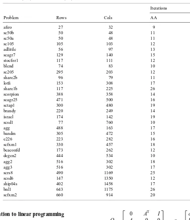
Table 1
The number of rows (Rows), columns (Cols) of test problems, as well as the number of iterations for Andersen (AA) and the method (KS) of Section 1
Iterations
Problem Rows Cols AA KS
aro 27 32 9 21
sc50b 50 48 11 18
sc50a 50 48 11 20
sc105 105 103 12 21
adlittle 56 97 13 24
scagr7 129 140 15 27
stocfor1 117 111 12 24
blend 74 83 10 24
sc205 295 203 12 23
share2b 96 79 11 27
lot 153 308 17 30
share1b 117 225 26 38
scorpion 388 358 14 21
scagr25 471 500 16 40
sctap1 300 480 19 32
brandy 220 249 14 30
israel 174 142 19 48
scsd1 77 760 10 25
agg 488 163 17 72
bandm 305 472 15 30
e226 223 282 16 35
scfxm1 330 457 18 38
beaconfd 173 262 12 25
degen2 444 534 10 27
agg2 516 302 18 34
agg3 516 302 17 35
scrs8 490 1169 25 59
scsd6 147 1350 12 27
ship04s 402 1458 17 25
bnl1 643 1175 26 78
scfxm2 660 914 20 41
5. Application to linear programming
LetA∈Rk×l; c∈Rlandb∈Rk, and consider the
following linear programming problem:
min
x∈Rl{c
Tx|Ax=b; x¿0} (5.1)
and its dual
max
y∈Rk; s∈R1{b
Ty|ATy+s=c; s¿0}: (5.2)
Optimality conditions for (5.1) – (5.2) may be stated by (1.1) with
Q=
0 AT I A 0 0
−cT bT 0
; q=
c b
0
; z=
x y s
and by nonnegativity constraints x¿0 ands¿0. To deal with the free variablesyand to solve the problem, we may proceed as described in Section 4.
enough accuracy to deal with ill conditioning of the matrixQSQT. We prescale the matrixAwith a
proce-dure that aims to equalize the norms of all rows and columns ofA close to 1. Thereafter, to initialize the iterations, we set all variables equal to ten. Our exper-imental code does not deal with simple bounds; i.e. all variables are nonnegative or free. We compare the results with a state of the art interior point code by Andersen and Andersen [1], wherefore a similar stop-ping criterion is employed in both codes. In particular, the vital requirement is that the absolute value of the relative duality gap|cTx−bTy|=(1 +|cTx|) is less than
10−8. Besides, both codes employ primal and dual
in-feasibility tolerances, which dier, because initializa-tion procedures dier. We require the norms of primal and dual infeasibility vectors relative to norms of b
andc;respectively, to be less than 10−6. For the step
size parameter, we use= 0:99.
The results are shown in Table 1 below. We obtain approximately twice as many iterations as compared with using MOSEK v1.0.beta [1]. Given that the latter code employs most known enhancements for primal–
dual infeasible interior point methods, we may regard our results quite satisfactory.
Acknowledgements
The authors wish to thank Erling Andersen for pro-viding them with the results obtained with MOSEK, as well as an anonymous referee for drawing their at-tention to infeasible problems. Financial support for this work is gratefully acknowledged from The Foun-dation for the Helsinki School of Economics.
References
[1] E.D. Andersen, K.D. Andersen, The MOSEK interior point optimizer for linear programming: an implementation of the homogeneous algorithm, in: H. Frenk, K. Roos, T. Terlaky, S. Zhang (Eds.), High Performance Optimization, Proceedings of the HPOPT-II Conference, 2000.